Using your remote AWS instance (Part II)
Using your remote AWS instance (Part II)
The goal of this hands-on session is to run you through a demonstration of using the command line on an Amazon Web Service (AWS) instance to do some familiar bioinformatics analysis. Our previous Section 1 of this lab covered how to launch your own AWS instance.
1. Logging in to an AWS instance from your local terminal
In Section 1 we also described the process of connecting to an AWS Elastic Compute Cloud (a.k.a. EC2) virtual machine instance (a.k.a computer in the cloud) through SSH. This is the same mechanism we would use to connect to any remote UNIX based computer.
However, due to the extra security protocols in place on AWS we needed to use a so-called keyfile along with our ssh command when we logged in. Note that normally when you access another UNIX based computer you will typically just provide a user-specific password to login. .
Side-Note: Cryptographic keys are a secure way to authenticate (i.e. login) without having to use passwords. They consist of a pair of files called the public key and private key: the public part can be shared with whoever you’d like to authenticate with (in our case, AWS!), and the private part is kept “secret” on your machine. In our particular case AWS stores the public part of the key pair which can be thought of as just like a house lock. You will download and use the private part of the key pair which can be thought of as just like a house key. You can read more about key cryptography here.
The private key for your instance was created and (hopefully) downloaded by you toward the end of Section 1 of this lab. You will need this private file together with the address of your instance that you copied from the AWS console in Section 1 to login again to your instance should you become disconected.
2. Update the software on the machine
At this point what you have connected to is effectively a brand new machine (with a fresh Ubuntu Linux OS just installed). Like any new machine it is a good idea to first update the software to make sure we are using the latest and greatest versions of the various software we will need later.
Copy and paste the following two commands into your AWS instance command line to updates the software list and then install NCBI BLAST+:
sudo apt-get update
sudo apt-get -y install ncbi-blast+
Please make sure to hit enter after the paste – sometimes the last line doesn’t paste completely.
The apt-get command is used to find, install and upgrade software packages on Debian based Linux machines like the one you are using here. The sudo in-front of these commands gives us administrator (or in UNIX speak ‘superuser’) permissions to install packages that a normal user does not have. The name sudo stands for “superuser do” as the early versions of sudo were designed to run commands only as the superuser.
Side-note: If you are using a Mac laptop ask Barry about the homebrew package manager for that OS which can do much of the same as apt-get but on a Mac. It is super useful!
3. Download some sequences to work with
First we need some data! Let’s grab the mouse and zebrafish RefSeq protein data sets from NCBI, and put them in a new directory that we will create called work. If you’ve just logged in, you should be in your home area already, but if you’re unsure, just run cd by itself and hit enter.
cd
mkdir work
cd work
Check you are where you think you are (i.e. in /home/ubuntu/work) with the Print Working Directory command, pwd:
pwd
Now, we’ll use curl to download the files:
curl -O ftp://ftp.ncbi.nih.gov/refseq/M_musculus/mRNA_Prot/mouse.1.protein.faa.gz

curl -O ftp://ftp.ncbi.nih.gov/refseq/M_musculus/mRNA_Prot/mouse.2.protein.faa.gz

curl -O ftp://ftp.ncbi.nih.gov/refseq/D_rerio/mRNA_Prot/zebrafish.1.protein.faa.gz
4. Inspect our sequences
If you look at the files in the current directory, you should see four files:
ls -l
should show you:
total 31416
-rw-rw-r-- 1 ubuntu ubuntu 11349404 Nov 20 20:16 mouse.1.protein.faa.gz
-rw-rw-r-- 1 ubuntu ubuntu  6867542 Nov 20 20:17 mouse.2.protein.faa.gz
-rw-rw-r-- 1 ubuntu ubuntu 13947543 Nov 20 20:17 zebrafish.1.protein.faa.gz
All three files are FASTA protein files (that’s what the .faa suggests) that are compressed with gzip (that’s what the .gz means).
Uncompress them:
gunzip *.faa.gz
Q. What does the star character accomplish here? Ask Barry, or your class neighbor, if you are not sure!
Now and let’s look at the first few sequences in one of the files:
head mouse.1.protein.faa
These are protein sequences in FASTA format. FASTA format is something many of you have probably seen in one form or another – it’s pretty ubiquitous. It’s a text file, containing records; each record starts with a line beginning with a ‘>’, and then contains one or more lines of sequence text.
Q. How many sequences are in this mouse.1.protein.faa file? Hint: Try using grep to figure this out…
Let’s take the first two sequences and save them to a new file that we will create called mm-first.fa. We’ll do this using output redirection with ‘>’, which says “take all the output and put it into this file here.”
head -11 mouse.1.protein.faa > mm-first.fa
Q. What happens if you run the above command without the > mm-first.fa part?
Q. What happens if you were to use two ‘>’ symbols (i.e. >> mm-first.fa)?
You can do less mm-first.fa to see the contents of that file (or more mm-first.fa). Type space-bar to move down and ‘q’ to get out of paging mode.
Maje sure you have run the correct command above with the one ‘>’ symbol so you only have two sequences in your new file.
Now let’s BLAST these two sequences against the entire zebrafish protein data set. First, we need to tell BLAST that the zebrafish sequences are (a) a database, and (b) a protein database. That’s done by calling ‘makeblastdb’:
makeblastdb -in zebrafish.1.protein.faa -dbtype prot
5. Running our first command line BLAST
Next, we call protein BLAST (blastp) to do the search:
blastp -query mm-first.fa -db zebrafish.1.protein.faa
This should run pretty quickly, but you’re going to get a lot of output!! To save it to a file instead of watching it go past on the screen, ask BLAST to save the output to a file that we’ll name mm-first.x.zebrafish.txt:
blastp -query mm-first.fa -db zebrafish.1.protein.faa -out mm-first.x.zebrafish.txt
and then you can ‘page’ through this file at your leisure by typing:
less mm-first.x.zebrafish.txt
(Type spacebar to move down, and ‘q’ to get out of paging mode.)
6. Running more BLAST jobs
Let’s do some more sequences (this one will take a little longer to run):
head -497 mouse.1.protein.faa > mm-second.fa
Q.How would you determine how many sequences are in the mm-second.fa file?
Now run BLAST with this file as a query and the zebrafish database
blastp -query mm-second.fa -db zebrafish.1.protein.faa -out mm-second.x.zebrafish.txt
This will compare the first 80 sequences. You can look at the output file with:
less mm-second.x.zebrafish.txt
(and again, type ‘q’ to get out of paging mode.)
7. Producing a TSV output
Last, but not least, let’s generate a more machine-readable version of these results:
blastp -query mm-second.fa -db zebrafish.1.protein.faa -out mm-second.x.zebrafish.tsv -outfmt 6
You can open the file with less mm-second.x.zebrafish.tsv to see how the file looks like.
See this link for a description of the possible BLAST output formats.
8. Transfer your results back to your computer
You now have a decision to make: do you want to further analyze your results on this remote machine or transfer your current working results back to your own machine for local analysis. Let’s do the later first and in so doing demonstrate how to transfer data between your remote AWS instance (i.e. remote server) and your local machine (i.e. your own laptop).
For data transfer we will first demonstrate the use of scp for Secure CoPy.
Back on your LOCAL machine in a new terminal go to a directory where you want to store the incoming data. For example, I am working in a directory on my Desktop called week10
# Use a location directory that exists and is meaningful for you!
cd ~/Desktop/week10
Now still on your local machine use scp to transfer the file or files you want copied across (N.B. You will need to substitute the IP address for the remote machine you are using for the YOUR_IP_ADDRESS in the command here just as we did with our initial login):
scp -i ~/Downloads/barry_bioinf.pem ubuntu@YOUR_IP_ADDRESS:~/work/mm-second.x.zebrafish.tsv .
Note. Like cp and similar tools, the source is always the first argument, and the destination is always the second argument.
9. Install R/RStudio on AWS!
If you want to analyze your data further on the remote machine (and why not, is likely bigger and faster after all) then we need to first install the software you want to use for the analysis you have in mind. The following section demonstrates how to install R and RStudio on your remote machine
9A. Install RStudio
The following commands install the prerequisites for RStudio Web, download the latest version, and then install it.
N.B. Make sure you are working on your remote AWS machine and not your local machine. To make sure try the command
whoamiwhich will tell you your login name. It should beubuntuif your terminal session is connected to AWS.
sudo apt-get update && sudo apt-get -y install gdebi-core r-base
After that finishes, download and install RStudio:
wget https://s3.amazonaws.com/rstudio-ide-build/server/bionic/amd64/rstudio-server-1.4.1043-amd64.deb
sudo gdebi rstudio-server-1.4.1043-amd64.deb
After answering yes when prompted you should see a final line indicating that an RStudio server has started:
You can double check with:
rstudio-server status
Push ‘q’ to exit and note that you should see a line saying “Active: active (running)”.
9B. Figure out your machines Web address to connect to.
Because we’re using the cloud to run things, everyone will have a different computer that they’re running RStudio on. We will use YOUR specific machines IP address to access YOUR specific RStudio server.
If you have forgotten your IP address you can use find it out like so:
curl ifconfig.me
This should print-out your IP address that will look something like 172.31.18.114. Lets assign this to a variable (called myip in this case) and use that to print out the web address you will use to access YOUR server:
myip=`curl ifconfig.me`
echo My RStudio Web server is running at: http://$myip:8787/
After running this, copy/paste the URL into your Web browser; you should see login page. Enter the username ubuntu. Unfortunately, we have not setup a password yet so you will need to return to the terminal and run:
sudo passwd ubuntu
to change your password for this instance.
You will be prompted to enter a new password:
Enter new UNIX password:
Retype new UNIX password:
but note that the text will not echo to the screen (because it’s a password!)
Return to the browser login page and enter the username: ubuntu and your new password that you just set. Note this will not change the global AWS login info (i.e. it only affects this instance).
Once RStudio is up and running, we’ll give you a quick tour of the RStudio Web interface, but essentially it is much the same as the Desktop version of RStudio that we have been using up till now. The big difference is that this RStudio is not running on your laptop but rather in the cloud ;-)
10. Using RStudio online (or locally) to read your output
If you are working on the remote machine you can use RStudio to open a New Project > Existing Directory and chose your work directory that contains your BLAST results.
If you are working on your own machine please open a new RStudio project where you are typically storing all your class work to date.
Now open an Rmarkdown document selecting html format and read your mm-second.x.zebrafish.tsv. Set the colnames to be:
c("qseqid", "sseqid", "pident", "length", "mismatch", "gapopen", "qstart", "qend", "sstart", "send", "evalue", "bitscore")
Make a histogram of the $bitscore values. You may want to set the optional breaks to be a larger number (e.g. breaks=30).
What do you notice here? Note that larger bitscores are better.
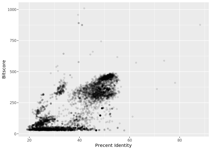
Is there a straightforward relationship between percent identity ($pident) and bitscore ($bitscore) for the alignments we generated?
The answer is that bitscores are only somewhat related to pident; they take into account not only the percent identity but the length of the alignment. You can get a napkin sketch estimate of this by doing the following:
## Asuming your blast results are stored in an object called 'b'
plot(b$pident  * (b$qend - b$qstart), b$bitscore)
Or using ggplot (note you will have to install the ggplot2 package first if you are working on AWS)
library(ggplot2)
ggplot(b, aes(pident, bitscore)) + geom_point(alpha=0.1)
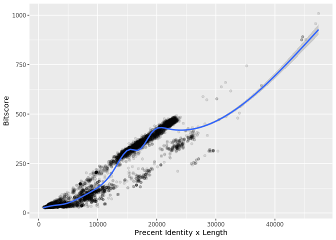
ggplot(b, aes((b$pident * (b$qend - b$qstart)), bitscore)) + geom_point(alpha=0.1) + geom_smooth()
Now Knit your Rmarkdown document and transfer everything back to YOUR LOCAL computer using scp as demonstrated in section 8 above.
# On your local machine
scp -i ~/Downloads/barry_bioinf.pem -r ubuntu@YOUR_IP_ADDRESS:~/work/* .
Q. Note the addition of the -r option here: What is it’s purpose? Also what about the *, what is it’s purpose here?
Using rsync
We could also use rsync to sync up your two directories both remote and local. Typical rsync use is like the following
# Example only...
rsync -a username@remote_host:/home/username/dir1 place_to_sync_on_local_machine
Which would look something like this for us
# Example only...
rsync -az ubuntu@149.165.170.49:~/work/ .
Again, like cp, scp and similar tools, the source is always the first argument, and the destination is always the second.
Because we have to supply the keyfile for security reasons our actual command is bit more convoluted for this example. Note that normally for machines you access you wont need this type of keyfile approach:
rsync -az -e "ssh -i ~/Downloads/barry_bioinf.pem" ubuntu@149.165.170.49:~/work/* .
There are lots of very useful options that you can supply to rsync including the -P and -z and –exclude options. Can you determine what they do? A useful resource here is the man page and of course on-line guides like this one
Notes:
if you are done you can Stop your AWS instance so we are not charged for it any longer. Go to the AWS console page and select your instance then click “Instance State” > “Stop Instance”.
you can execute multiple commands at a time;
You might see a warning -
Selenocysteine (U) at position 310 replaced by Xwhat does this mean?
why did it take longer to BLAST
mm-second.fathanmm-first.fa?when we plot e-values why do you often work in -log(evalue) units?
what is an advantage of
rsyncoverscp?what is the advantage of using R (and other tools) on remote machines vs our local computer?
what is the disadvantage of remote vs local work?
Things for Barry to mention and discuss:
blastpoptions and -help.- command line options, more generally - why so many?
- automation rocks!
Other topics to discuss:
- when you shut down a VM, you lose all your data
- what computer(s) is this all happening on?
> OPTIOPNAL…
Next we’re going to become more familiar with running longer programs and analysis work-flows on the command line.