Visualization with R Lecture (Part 2)
Background
This document contains all the code used to generate the images for lecture number 8 of BGGN-213 (Foundations of Bioinformatics) and follows on from Part 1.. This document is not meant to stand alone – it has very little explanatory text. It is meant to be a reference for students who want to see how the plots for the presentation were made.
Setup
First I set up a theme for presentations. It uses white on black (good for large, dimly lit rooms), and lines and text that are too small/fine when rendered in a document, but which work well when rendered at 300dpi for the presnetation. Note that I would usually not use white on black for documents, but I use this as the default theme throughout because there isn’t an easy way (that I know of) to set the default color of a geom to something other than black.
theme_preso <- theme_dark(base_size=11)
##theme_set(theme_preso)

preso_save<-function(filename, plot=last_plot(), theme=theme_preso,
                     width=1280/300, height=720/300, dpi=300) {
  ggsave(filename, ##plot+theme,
         width=width, height=height, dpi=dpi)
}
Part 1: Why visualize at all?
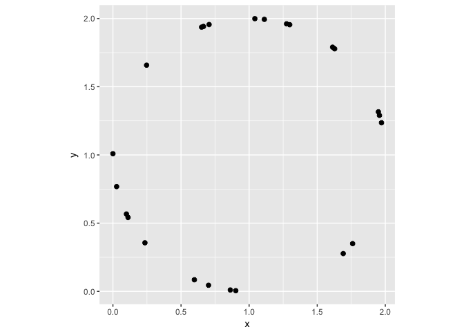
A circle
Showing the data in a scatterplot makes the relationship obivous pre-attentively.
circle<-read.delim(textConnection(
"x  y
1.972   1.236
1.112   1.994
0   1.009
0.665   1.942
0.235   0.356
0.247   1.658
1.275   1.961
0.702   0.045
1.76    0.35
1.691   0.277
1.628   1.778
1.957   1.29
0.111   0.542
0.902   0.005
0.598   0.085
1.613   1.79
1.298   1.955
0.651   1.937
1.949   1.316
0.099   0.567
0.862   0.01
0.027   0.768
0.706   1.956
1.042   1.999"))

ggplot(circle, aes(x,y))+geom_point(color="black", size=2)+coord_equal()
preso_save("img/circle.png")
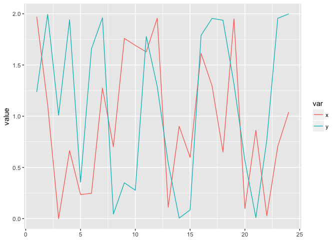
But showing it as a time-series obscures the relationship. This is arguably worse than a simple table.
circle_w <- circle %>%
  mutate(n=1:nrow(circle)) %>%
  gather(var, value, x, y)
ggplot(circle_w, aes(n, value, color=var))+geom_line()+xlab(NULL)
preso_save("img/circle_lines.png")
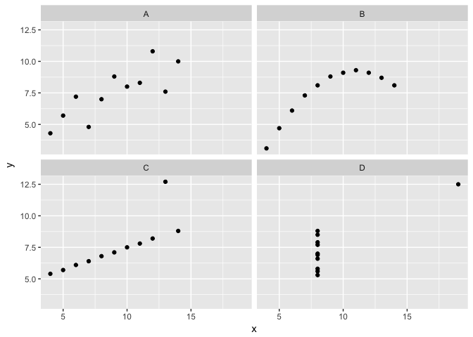
Anscombe’s Quartet
quartet<-read.delim(textConnection(
"group  x   y
A   10  8
A   8   7
A   13  7.6
A   9   8.8
A   11  8.3
A   14  10
A   6   7.2
A   4   4.3
A   12  10.8
A   7   4.8
A   5   5.7
B   10  9.1
B   8   8.1
B   13  8.7
B   9   8.8
B   11  9.3
B   14  8.1
B   6   6.1
B   4   3.1
B   12  9.1
B   7   7.3
B   5   4.7
C   10  7.5
C   8   6.8
C   13  12.7
C   9   7.1
C   11  7.8
C   14  8.8
C   6   6.1
C   4   5.4
C   12  8.2
C   7   6.4
C   5   5.7
D   8   6.6
D   8   5.8
D   8   7.7
D   8   8.8
D   8   8.5
D   8   7
D   8   5.3
D   19  12.5
D   8   5.6
D   8   7.9
D   8   6.9"))
All four are identical on common statistical measures.
quartet %>%
  group_by(group) %>%
  summarize(mean_x=mean(x), mean_y=mean(y))
## # A tibble: 4 x 3
##    group mean_x   mean_y
##   <fctr>  <dbl>    <dbl>
## 1      A      9 7.500000
## 2      B      9 7.490909
## 3      C      9 7.500000
## 4      D      9 7.509091
quartet %>%
  group_by(group) %>%
  do(tidy(lm(y~x, data=.))) %>%
  select(group, term, estimate) %>%
  spread(term, estimate)
## # A tibble: 4 x 3
## # Groups:   group [4]
##    group `(Intercept)`         x
## * <fctr>         <dbl>     <dbl>
## 1      A      3.008182 0.4990909
## 2      B      2.990909 0.5000000
## 3      C      3.016364 0.4981818
## 4      D      3.017273 0.4990909
quartet %>%
  group_by(group) %>%
  do(glance(lm(y~x, data=.))) %>%
  select(group, r.squared)
## # A tibble: 4 x 2
## # Groups:   group [4]
##    group r.squared
##   <fctr>     <dbl>
## 1      A 0.6709131
## 2      B 0.6641054
## 3      C 0.6694547
## 4      D 0.6740641
But obivously different visually.
ggplot(quartet, aes(x,y))+geom_point(color="black")+facet_wrap(~group)
preso_save("img/anscombe.png")
Part 2: Estimation
The hierarchy
The first rule of color is do not talk about color
Color has three separate channels.
values<-data.frame(val=1:5, y=1)

theme_extras <- theme(axis.title=element_blank(),
                      axis.text=element_blank(),
                      axis.ticks=element_blank(),
                      legend.position="none")

ggplot(values, aes(val,y,fill=val)) + geom_tile() + scale_fill_gradient(low="black", high="white", limits=c(0,6)) + theme_extras
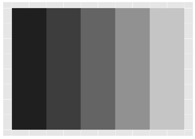
preso_save("img/luminance.png", height=720/300/3, theme=theme_preso + theme_extras)
ggplot(values, aes(val,y,fill=val)) + geom_tile() + scale_fill_gradient(low="white", high="red", limits=c(0,6)) + theme_extras
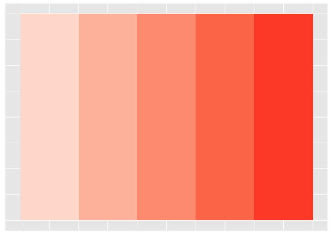
preso_save("img/saturation.png", height=720/300/3, theme=theme_preso + theme_extras)
ggplot(values, aes(val,y,fill=factor(val))) + geom_tile() + scale_fill_discrete() + theme_extras
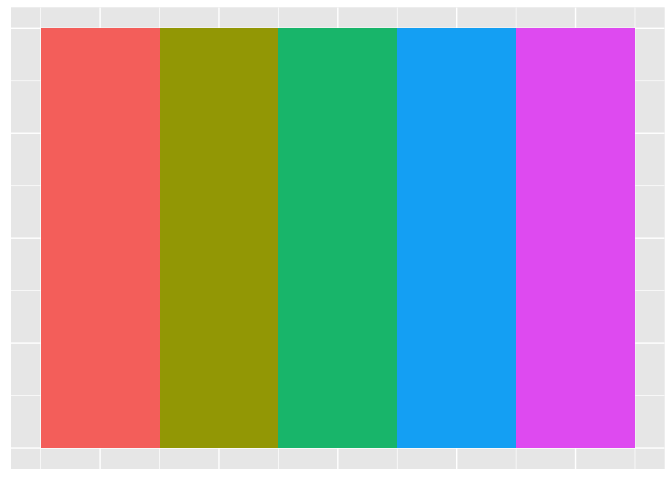
preso_save("img/hue.png", height=720/300/3, theme=theme_preso + theme_extras)
Lots of plots with the mtcars dataset. I had to drop the font size way down to get the plots the render well for the presentation. They are much too small for the document. I offer my apologies.
# Make model an actual column in the dataset.
mtcars <- mtcars %>%
  mutate(model=rownames(mtcars))
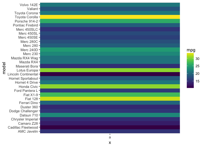
Hue
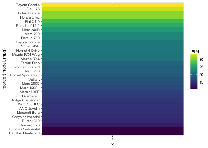
The viridis hue scale. I didn’t end up using this in the presentation. I probably should have, as it’s far superior to the crappy one I made up.
ggplot(mtcars, aes("a", model, fill=mpg))+geom_tile()+scale_fill_viridis()
ggplot(mtcars, aes("a", reorder(model, mpg), fill=mpg))+geom_tile()+scale_fill_viridis()
Ordered and unordered plots with hue encoding efficiency.
theme_extras <- theme(axis.title.x=element_blank(),
                      axis.text.x=element_blank(),
                      axis.ticks.x=element_blank(),
                      axis.text.y=element_text(size=rel(0.6)))

ggplot(mtcars, aes("a", model, fill=mpg)) +
  geom_tile() +
    scale_fill_gradient2(midpoint=median(mtcars$mpg), mid="#ffffbf", low="#91bfdb", high="#fc8d59") +
  # Terrible for color blind people
  #    scale_fill_gradient2(midpoint=median(mtcars$mpg), mid=muted("green")) +
  ylab(NULL) + theme_extras
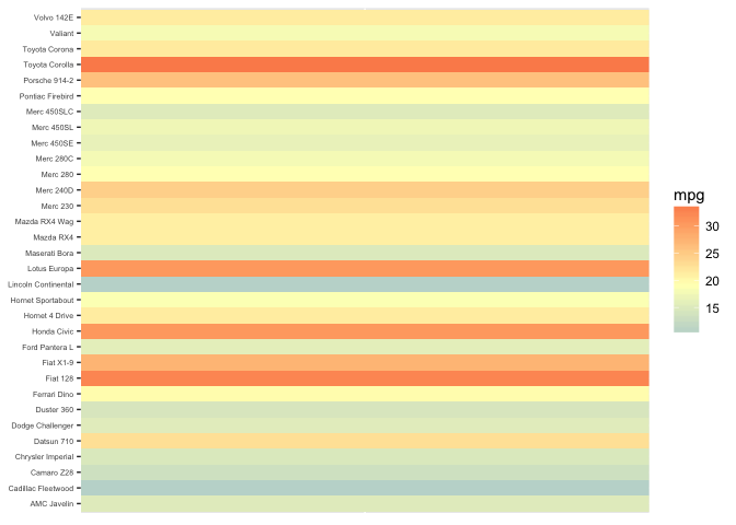
preso_save("img/mtcars_hue.png", width=1280/300*(3/4), theme=theme_preso+theme_extras)

ggplot(mtcars, aes("a", reorder(model, mpg), fill=mpg)) +
  geom_tile() +
    scale_fill_gradient2(midpoint=median(mtcars$mpg), mid="#ffffbf", low="#91bfdb", high="#fc8d59") +
  # Terrible for color blind people
  #    scale_fill_gradient2(midpoint=median(mtcars$mpg), mid=muted("green")) +
  ylab(NULL) + theme_extras
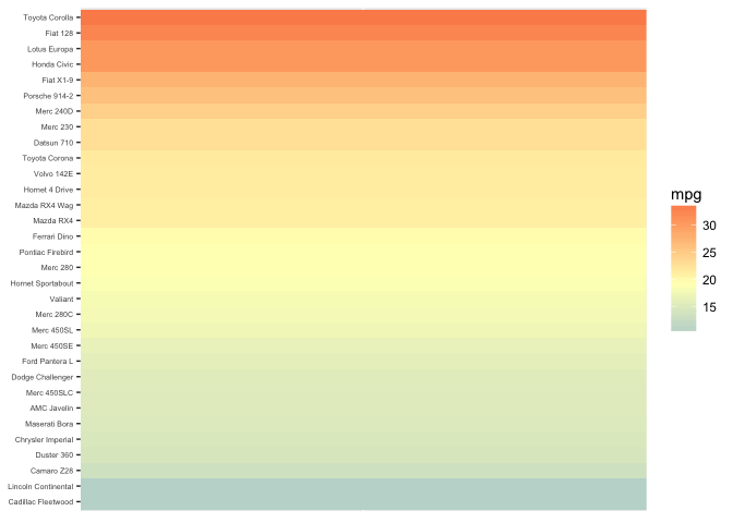
preso_save("img/mtcars_hue_ordered.png", width=1280/300*(3/4), theme=theme_preso+theme_extras)
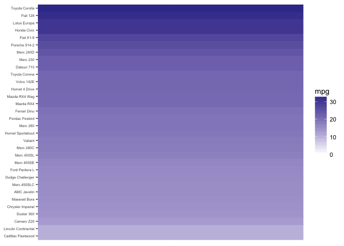
Saturation
Unordered and ordered plots with saturation.
ggplot(mtcars, aes("a", model, fill=mpg)) +
  geom_tile() +
  scale_fill_gradient(low="white", high=muted("blue"))+
  ylab(NULL) + theme_extras
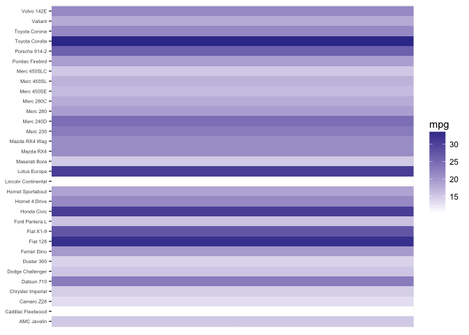
preso_save("img/mtcars_saturation.png", width=1280/300*(3/4), theme=theme_preso+theme_extras)

ggplot(mtcars, aes("a", reorder(model, mpg), fill=mpg)) +
  geom_tile() +
  scale_fill_gradient(low="white", high=muted("blue"))+
  ylab(NULL) + theme_extras
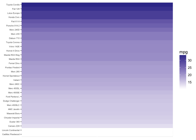
preso_save("img/mtcars_saturation_ordered.png", width=1280/300*(3/4), theme=theme_preso+theme_extras)
For accurate ratioing with saturation, the scale has to extend to zero.
ggplot(mtcars, aes("a", reorder(model, mpg), fill=mpg)) +
  geom_tile() +
  scale_fill_gradient(low="white", high=muted("blue"))+
  ylab(NULL) + theme_extras + expand_limits(fill=0)
preso_save("img/mtcars_saturation_expanded.png", width=1280/300*(3/4), theme=theme_preso+theme_extras)
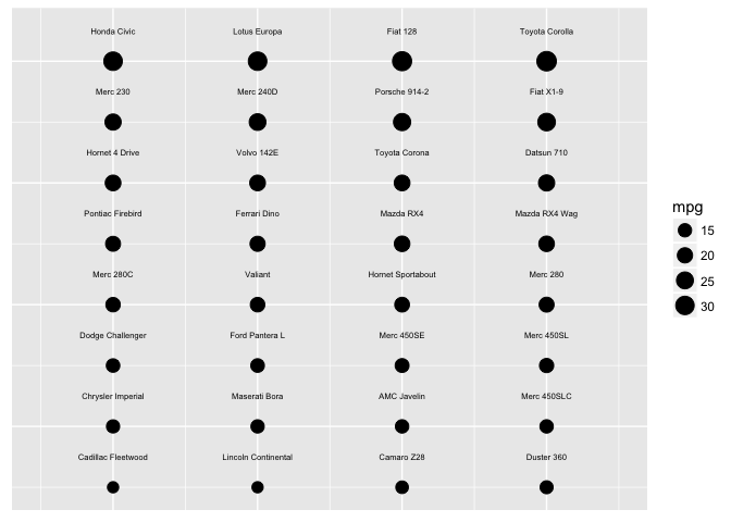
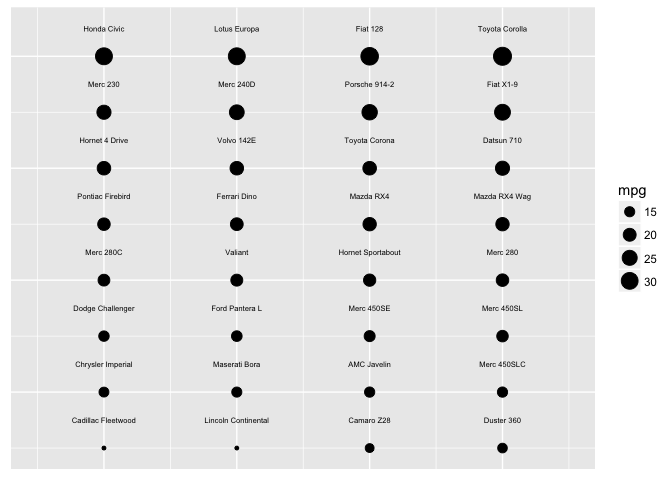
Area
mtcars <- mtcars %>%
  mutate(model=reorder(model, mpg)) %>%
  arrange(mpg, model)

theme_extras <- theme(axis.title=element_blank(),
                      axis.text=element_blank(),
                      axis.ticks=element_blank())

cols<-4
ggplot(mtcars, aes(rep(1:cols, 32/cols), rep(1:(32/cols), each=cols))) +
  geom_point(aes(size=mpg), color="black") +
  geom_text(aes(label=model), color="black", position=position_nudge(y=0.5), size=2) +
  expand_limits(x=c(0.5,4.5), y=c(1,8.5))+ ylab(NULL) + scale_size_area() + theme_extras
preso_save("img/mtcars_area.png", theme=theme_preso+theme_extras)
Again, accurate ratioing depends on a scale that goes to zero.
ggplot(mtcars, aes(rep(1:cols, 32/cols), rep(1:(32/cols), each=cols))) +
  geom_point(aes(size=mpg), color="black") +
  geom_text(aes(label=model), color="black", position=position_nudge(y=0.5), size=2) +
  expand_limits(x=c(0.5,4.5), y=c(1,8.5), size=15)+ ylab(NULL) + theme_extras
preso_save("img/mtcars_area_nonzero.png", theme=theme_preso+theme_extras)
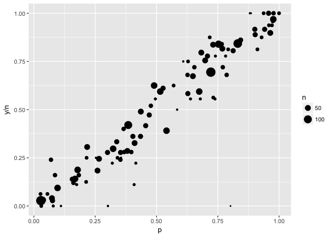
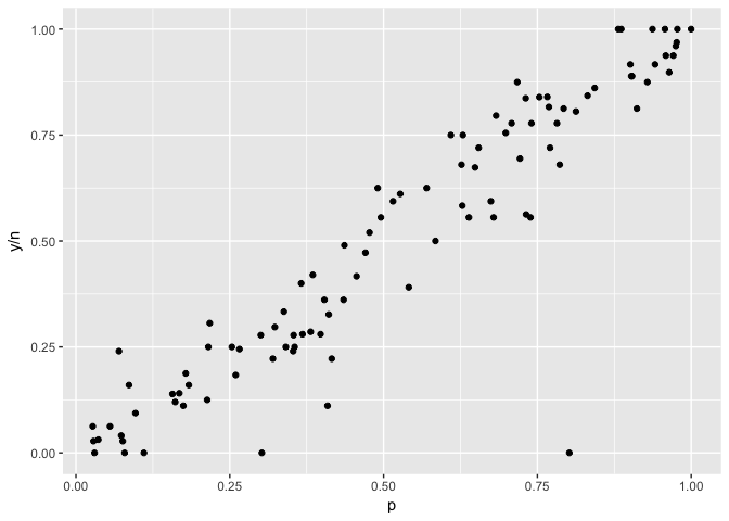
“Bubble charts” use size to indicate the weight of a point. In these plots the outliers have low weight (small size).
to_plot<-data.frame(p=runif(100),
                    n=rpois(100, 5)^2) %>%
  mutate(y=rbinom(100,n,p))
ggplot(to_plot,aes(p,y/n,size=n)) +geom_point(color="black") +scale_size_area()
ggplot(to_plot,aes(p,y/n)) +geom_point(color="black")
to_plot<-data.frame(trial=1:100,
                    n=rpois(100, 5)^2) %>%
  mutate(y=rbinom(100,n,0.5)/n)
ggplot(to_plot, aes(trial, y)) + geom_point(color="black")
## Warning: Removed 1 rows containing missing values (geom_point).
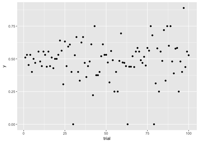
preso_save("img/flips_same.png")
## Warning: Removed 1 rows containing missing values (geom_point).
ggplot(to_plot, aes(trial, y, size=n)) + geom_point(color="black", alpha=2/3) + scale_size_area()
## Warning: Removed 1 rows containing missing values (geom_point).
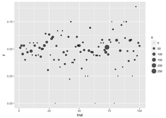
preso_save("img/flips_area.png")
## Warning: Removed 1 rows containing missing values (geom_point).
Angle
Again, note that the scale goes to zero (a horizontal line).
make_segment <- function(df, scale_low, scale_high) {
  scale_range <- scale_high-scale_low
  fraction <- (df$mpg-scale_low) / scale_range
  theta <- fraction * pi/2
  return(data.frame(x=c(0, cos(theta)),
                    y=c(0, sin(theta))))
}
mtcars_angle <- mtcars %>%
  group_by(model) %>%
  do(make_segment(., 0, max(mtcars$mpg)))
#  do(make_segment(., min(mtcars$mpg), max(mtcars$mpg)))

theme_extras <- theme(axis.title=element_blank(),
                      axis.text=element_blank(),
                      axis.ticks=element_blank(),
                      strip.text.x = element_text(size=rel(0.5), hjust=0))

ggplot(mtcars_angle, aes(x,y,group=model))+
  geom_path(color="black")+
  facet_wrap(~model,ncol=8)+coord_equal() +
  theme_extras
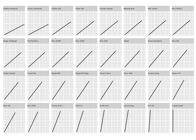
preso_save("img/mtcars_slope.png", theme=theme_preso+theme_extras)
Length
In the presentation, I use the jittered bars, so that the audience can’t rely on a common scale (which is next in the hierarchy).
theme_extras <- theme(axis.text.y=element_text(size=rel(0.7)),
                      axis.title.x=element_blank(),
                      axis.text.x=element_blank(),
                      axis.ticks.x=element_blank())

mtcars$random <- runif(32,0,5)
ggplot(mtcars, aes(x=random, xend=mpg+random, y=model, yend=model)) +
  geom_segment(size=2, color="black") + xlab(NULL) + ylab(NULL) + theme_extras
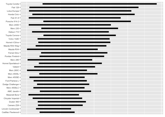
preso_save("img/mtcars_length.png", theme=theme_preso+theme_extras)


theme_extras <- theme(axis.text.y=element_text(size=rel(0.7)))

ggplot(mtcars, aes(x=0, xend=mpg, y=model, yend=model)) +
  geom_segment(size=2, color="black") + xlab(NULL) + ylab(NULL) + theme_extras
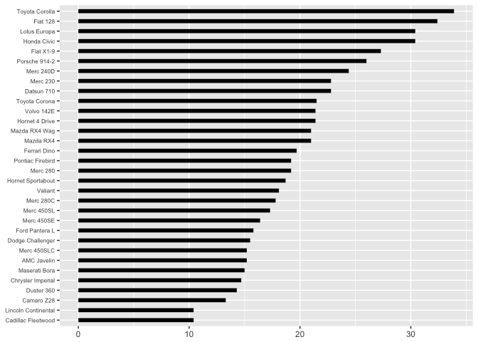
preso_save("img/mtcars_bars.png", theme=theme_preso+theme_extras)
Error bars encode information using length not on a common scale.
trials<-10
flips<-data.frame(trial=1:trials) %>%
  mutate(n=round(runif(trials, 20, 500)),
         y=rbinom(trials, n, 0.5),
         p=y/n,
         se=sqrt(p*(1-p)/n),
         lower=p-1.96*se,
         upper=p+1.96*se)
ggplot(flips, aes(trial, p, ymin=lower, ymax=upper)) + geom_pointrange(color="black")
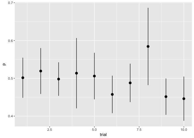
preso_save("img/flips.png")
Position on non-aligned scales
Doing this with facets is the easiest way in ggplot, but uses too much space.
theme_extras <- theme(axis.title.y=element_blank(),
                      axis.text.y=element_blank(),
                      axis.ticks.y=element_blank(),
                      strip.text.x = element_text(size=rel(0.5), hjust=0),
                      panel.grid.major =   element_line(colour = "grey50", size = 0.2),
                      panel.grid.minor =   element_line(colour = "grey50", size = 0.2, linetype="dotted")
                      )

ggplot(mtcars, aes(x=mpg, y="a")) + geom_point(color="black", size=1) +
  scale_x_continuous(breaks=c(10,20,30)) +
  facet_wrap(~model, ncol=8) + theme_extras
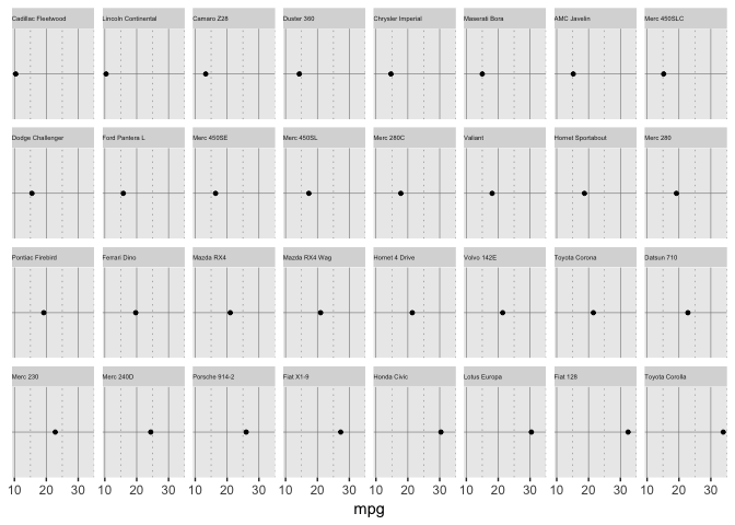
preso_save("img/mtcars_nonaligned.png", theme=theme_preso+theme_extras)
Position on a common scale
Ahhhh…
theme_extras <- theme(axis.text.y=element_text(size=rel(0.7)),
                      axis.title.y=element_text(size=rel(0.7)),
                      panel.grid.major =   element_line(colour = "grey20", size = 0.2))

ggplot(mtcars, aes(x=mpg, y=model)) +
  geom_point(color="black") +
  theme_extras + ylab(NULL)
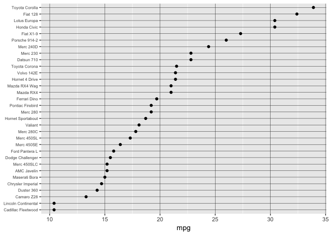
preso_save("img/mtcars_aligned.png", theme=theme_preso+theme_extras)
Ordering still crucial.
mtcars$model2<-factor(as.character(mtcars$model))
ggplot(mtcars, aes(x=mpg, y=model2)) +
  geom_point(color="black") +
  theme_extras + ylab(NULL)
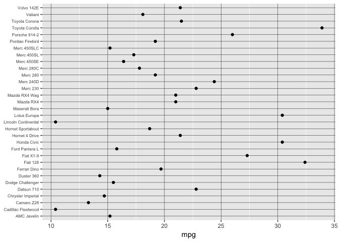
preso_save("img/mtcars_aligned_alpha.png", theme=theme_preso+theme_extras)
Dropping the scale to zero is a mistake here, lowers resolution and isn’t needed for accurate ratioing.
ggplot(mtcars, aes(x=mpg, y=model)) +
  geom_point(color="black") +
  theme_extras + ylab(NULL) + expand_limits(x=0)
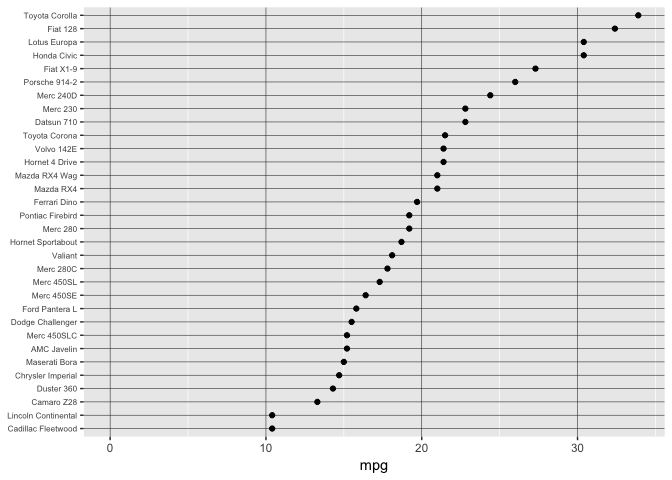
preso_save("img/mtcars_aligned_zero.png", theme=theme_preso+theme_extras)
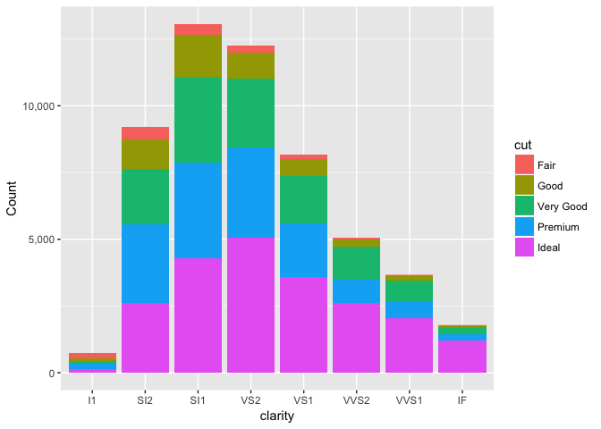
Observations
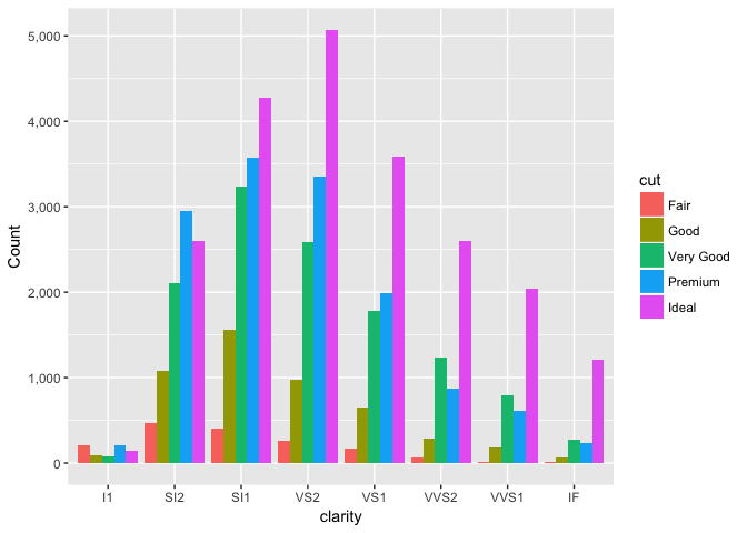
Stacked anything is nearly always a mistake
A stacked bar chart does two things, neither of the well.
ggplot(diamonds, aes(clarity, fill=cut, group=cut)) +
  geom_bar(stat="count", position="stack") +
  scale_y_continuous("Count", labels=comma)
preso_save("img/diamonds_stack.png")
The first is the total in each group.
diamonds_summary<-diamonds %>%
  group_by(clarity) %>%
  summarize(n=length(clarity))

ggplot(diamonds_summary, aes(clarity, n)) +
  geom_line(group=1, color="black") +
  geom_point(color="black") +
  expand_limits(y=0) +
  scale_y_continuous("Count", labels=comma)
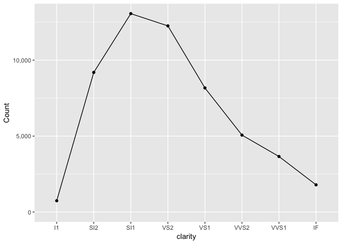
preso_save("img/diamonds_overall.png")
The second in the total in each combination, which is better shown with a parallel coordinates plot.
diamonds_summary2<-diamonds %>%
  group_by(clarity, cut) %>%
  summarize(n=length(clarity))

ggplot(diamonds_summary2, aes(clarity, n, color=cut, group=cut)) +
  geom_line() +
  geom_point() +
  expand_limits(y=0) +
  scale_y_continuous("Count", labels=comma)
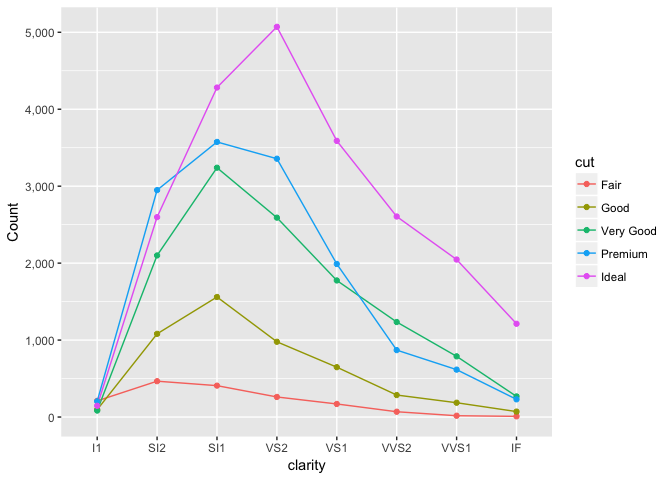
preso_save("img/diamonds_freqpoly.png")
Some phone data (from wikipedia).
phone_data<-
"Quarter    Windows Mobile  RIM Symbian iOS Android Bada    Windows Phone   Other
2016 Q2[39] 0   400.4   0   44395   296912  0   1971    680.6
2016 Q1[40] 0   660 0   51630   293771  0   2400    791
2015 Q4[41] 0   906.9   0   71526   325394  0   4395    887.3
2015 Q3[42] 0   977 0   46062   298797  0   5874    1133.6
2015 Q2[43] 0   1153    0   48086   271010  0   8198    1229
2015 Q1[44] 0   1325    0   60177   265012  0   8271    1268
2014 Q4[45] 0   1734    0   74832   279058  0   10425   1286.9
2014 Q3[46] 0   2420    0   38187   254354  0   9033    1310.2
2014 Q2[47] 0   2044    0   35345   243484  0   8095    2044
2014 Q1[44] 0   1714    0   43062   227549  0   7580    1371
2013 Q4[48] 0   1807    0   50224   219613  0   8534    1994
2013 Q3[49] 0   4401    458 30330   205023  633 8912    475
2013 Q2[50] 0   6180    631 31900   177898  838 7408    472
2013 Q1[51] 0   6219    1349    38332   156186  1371    5989    600
2012 Q4[52] 0   7333    2569    43457   144720  2684    6186    713
2012 Q3[53] 0   8947    4405    23550   122480  5055    4058    684
2012 Q2[54] 0   7991    9072    28935   98529   4209    4087    863
2012 Q1[55] 0   9939    12467   33121   81067   3842    2713    1243
2011 Q4[56] 0   13185   17458   35456   75906   3111    2759    1167
2011 Q3[57] 0   12701   19500   17295   60490   2479    1702    1018
2011 Q2[58] 0   12652   23853   19629   46776   2056    1724    1051
2011 Q1 982 13004   27599   16883   36350   1862    1600    1495
2010 Q4[56] 3419    14762   32642   16011   30801   2027    0   1488
2010 Q3[57] 2204    12508   29480   13484   20544   921 0   1991
2010 Q2[58] 3059    11629   25387   8743    10653   577 0   2011
2010 Q1[59] 3696    10753   24068   8360    5227    0   0   2403
2009 Q4[60] 4203    10508   23857   8676    4043    0   0   2517
2009 Q3[61] 3260    8523    18315   7040    1425    0   0   2531
2009 Q2[62] 3830    7782    20881   5325    756 0   0   2398
2009 Q1[63] 3739    7534    17825   3848    575 0   0   2986
2008 Q4[64] 4714    7443    17949   4079    639 0   0   3319
2008 Q3[65] 4053    5800    18179   4720    0   0   0   3763
2008 Q2[66] 3874    5594    18405   893 0   0   0   3456
2008 Q1[64] 3858    4312    18400   1726    0   0   0   4113
2007 Q4[64] 4374    4025    22903   1928    0   0   0   3536
2007 Q3[65] 4180    3192    20664   1104    0   0   0   3612
2007 Q2[66] 3212    2471    18273   270 0   0   0   3628
2007 Q1[64] 2931    2080    15844   0   0   0   0   4087"
phones<-read.delim(textConnection(phone_data))
phones <- phones %>%
  mutate(Other = Other + Bada + Windows.Phone,
         Bada = NULL,
         Windows.Phone = NULL,
         Quarter = str_replace(Quarter, "\\[\\d+\\]", ""),
         Year = as.integer(str_split_fixed(Quarter, " ", 2)[,1]),
         Quarter = str_split_fixed(Quarter, " ", 2)[,2],
         qtr = as.integer(str_replace(Quarter, "Q", "")),
         year = Year+0.25*(qtr-1)) %>%
  gather(os, ct, -Year, -Quarter, -qtr, -year) %>%
  mutate(ct = as.numeric(ct)) %>%
  group_by(year) %>%
  mutate(share = ct/sum(ct))
phones
## # A tibble: 228 x 7
## # Groups:   year [38]
##    Quarter  Year   qtr    year             os    ct share
##      <chr> <int> <int>   <dbl>          <chr> <dbl> <dbl>
##  1      Q2  2016     2 2016.25 Windows.Mobile     0     0
##  2      Q1  2016     1 2016.00 Windows.Mobile     0     0
##  3      Q4  2015     4 2015.75 Windows.Mobile     0     0
##  4      Q3  2015     3 2015.50 Windows.Mobile     0     0
##  5      Q2  2015     2 2015.25 Windows.Mobile     0     0
##  6      Q1  2015     1 2015.00 Windows.Mobile     0     0
##  7      Q4  2014     4 2014.75 Windows.Mobile     0     0
##  8      Q3  2014     3 2014.50 Windows.Mobile     0     0
##  9      Q2  2014     2 2014.25 Windows.Mobile     0     0
## 10      Q1  2014     1 2014.00 Windows.Mobile     0     0
## # ... with 218 more rows
All rules have exceptions. A stacked area chart with phone data is ok because it makes the point more effectively.
ggplot(phones, aes(year, share, group=os, fill=os)) + geom_area()
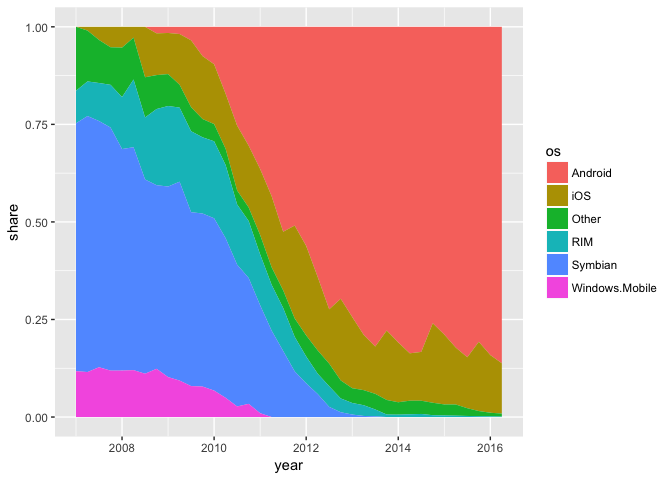
preso_save("img/phones_area.png")
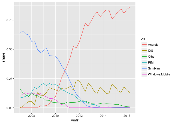
The line chart is weaker.
ggplot(phones, aes(year, share, group=os, color=os)) + geom_line()
Growth charts usually aren’t
This stacked area chart sucks.
library(gapminder)
continent_pop <- gapminder %>%
  group_by(continent, year) %>%
  summarize(pop=sum(as.numeric(pop))) %>%
  ungroup()
ggplot(continent_pop, aes(year, pop/1e9, group=continent, fill=continent)) +
  geom_area() +
  scale_y_continuous("Population (Billions)", labels=comma) +
  scale_color_brewer(type="qual", palette=1) + xlab(NULL)
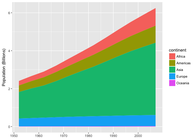
preso_save("img/population_area.png")
This line chart isn’t much better if you care about growth rates, becuse growth is encoded with angle (slope).
ggplot(continent_pop, aes(year, pop/1e9, group=continent, color=continent)) +
  geom_line() + scale_y_log10("Population (Billions)", labels=comma) +
  scale_color_brewer(type="qual", palette=1) + xlab(NULL)
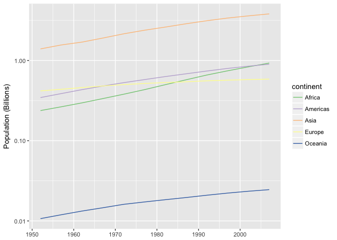
preso_save("img/population.png")
If growth is important, take derivatives and plot growth directly on the y-axis.
continent_pop <- continent_pop %>%
  group_by(continent) %>%
  arrange(year) %>%
  mutate(growth=c(NA,diff(pop)))
ggplot(continent_pop, aes(year, growth/pop, group=continent, color=continent)) +
  geom_line() + scale_color_brewer(type="qual", palette=1) +
  xlab(NULL) + scale_y_continuous("Pct. Growth", labels=percent)
## Warning: Removed 5 rows containing missing values (geom_path).
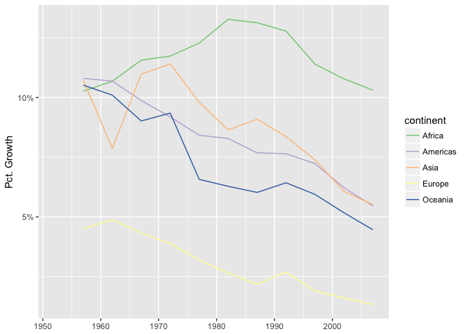
preso_save("img/population_growth.png")
## Warning: Removed 5 rows containing missing values (geom_path).
Putting the data on a common scale helps tremendously
host_dat = data.frame(t=seq.POSIXt(as.POSIXct("2016-06-01 00:00:00"),
                                   as.POSIXct("2016-06-01 01:00:00"),
                                   by=30)) %>%
  mutate(cpu=rnorm(length(t), 40, 5),
         latency=rnorm(length(t), 4, 0.1))

host_dat$cpu[50] = 100
host_dat$latency[60] = host_dat$latency[60]*3

host_dat_w <- host_dat %>%
  gather(var, value, -t) %>%
  group_by(var) %>%
  mutate(std_value = (value-mean(value))/sd(value))
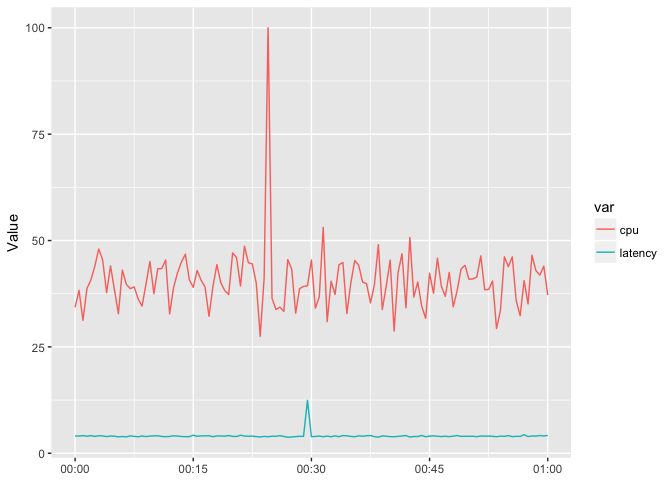
The user has to work to see if the peaks are aligned.
ggplot(host_dat_w, aes(t, value)) + geom_line(color="black") +
  facet_wrap(~var, scales="free") + xlab(NULL)
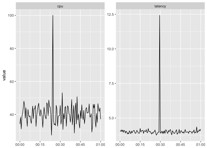
preso_save("img/cpu_latency_nonaligned.png")
You want to put them on the same scale, but the magnitude of the series is different.
ggplot(host_dat_w, aes(t, value, color=var, group=var)) +
  geom_line() + xlab(NULL) + ylab("Value")
preso_save("img/cpu_latency_aligned.png")
So “standardize” them by suntracting the mean and dividing by the standard deviation.
ggplot(host_dat_w, aes(t, std_value, color=var, group=var)) +
  geom_line() + xlab(NULL) + ylab("Standardized Value")
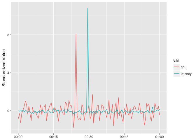
preso_save("img/cpu_latency_std_aligned.png")
TODO: Show deseasonalizing too (usually easy and automatic if many seasonal cycles are available).
Scatter plots show relationships directly
dat <- data.frame(x=seq(1,6*pi,length.out = 100))
# Two series, noe of which varies with the square, the other linearly
dat <- dat %>%
  mutate(Dependency=1.4+sin(x),
         Service=(1.1+sin(x))^2)
# Jitter the points
dat <- dat %>%
  mutate(Service=rnorm(length(x), mean = Service, sd=Service/10),
         Dependency=rnorm(length(x), mean = Dependency, sd=Dependency^(2/3)/10))
# Put in long format
dat_l <- dat %>%
  gather(var, value, -x)
They move together, but what, preciscely is the nature of the relationship?
ggplot(dat_l, aes(x, value))+geom_line(color="black")+facet_wrap(~var, scales="free")
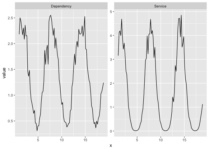
preso_save("img/ts_vs_scatter_facet.png")
ggplot(dat_l, aes(x, value, color=var))+geom_line()
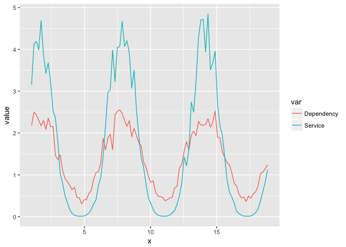
preso_save("img/ts_vs_scatter_ts.png")
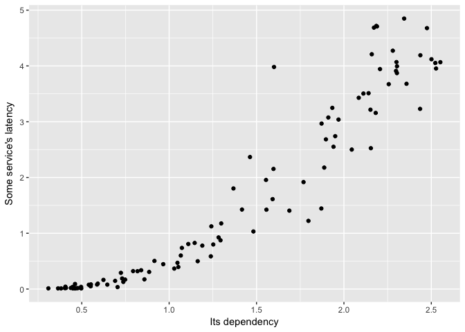
A scatterplot is more revealing.
ggplot(dat, aes(Dependency, Service)) + geom_point(color="black") +
  ylab("Some service's latency") + xlab("Its dependency")
preso_save("img/ts_vs_scatter_scatter.png")
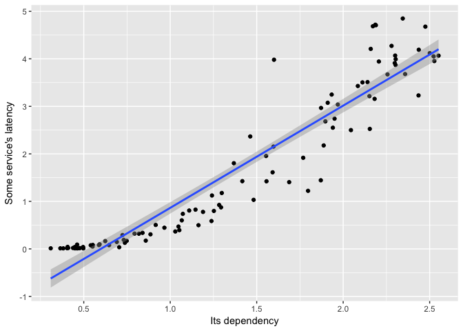
It’s clear that the relationship isn’t linear.
ggplot(dat, aes(Dependency, Service))+geom_point(color="black")+geom_smooth(method="lm") +
  ylab("Some service's latency") + xlab("Its dependency")
preso_save("img/ts_vs_scatter_lm.png")
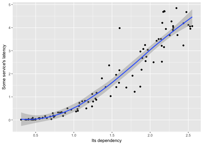
A loess fit looks nice.
ggplot(dat, aes(Dependency, Service))+geom_point(color="black")+geom_smooth(method="loess") +
  ylab("Some service's latency") + xlab("Its dependency")
preso_save("img/ts_vs_scatter_loess.png")
Part 3: Assembly
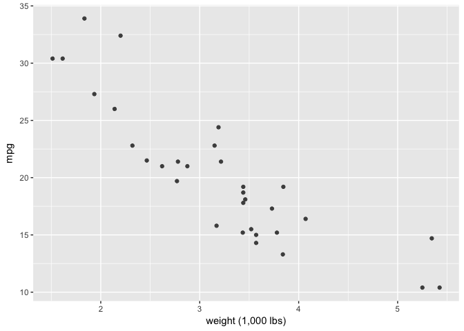
The Law of Continuity
The circle from the start is a good example, as is a simple scatterplot. Note that the continuity just has to be suggestive, not perfect.
ggplot(mtcars, aes(wt, mpg)) +
  geom_point(color="black") +
  xlab("weight (1,000 lbs)")

preso_save("img/wt_mpg_scatter.png")
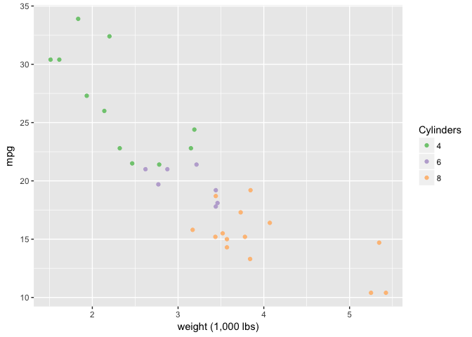
The Law of Similarity
Color is pretty good.
# Make number of cylinders a factor, so ggplot will choose a discrete scale.
mtcars$cyl<-factor(mtcars$cyl)

ggplot(mtcars, aes(wt, mpg)) +
  geom_point(aes(color=cyl)) +
  xlab("weight (1,000 lbs)") +
  scale_color_brewer("Cylinders", type="qual", palette=1)
preso_save("img/wt_mpg_scatter_color.png")
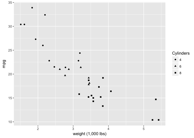
These filled shapes aren’t great.
ggplot(mtcars, aes(wt, mpg)) +
  geom_point(aes(shape=cyl), color="black") +
  xlab("weight (1,000 lbs)") +
  scale_shape("Cylinders")
preso_save("img/wt_mpg_scatter_shape1.png")
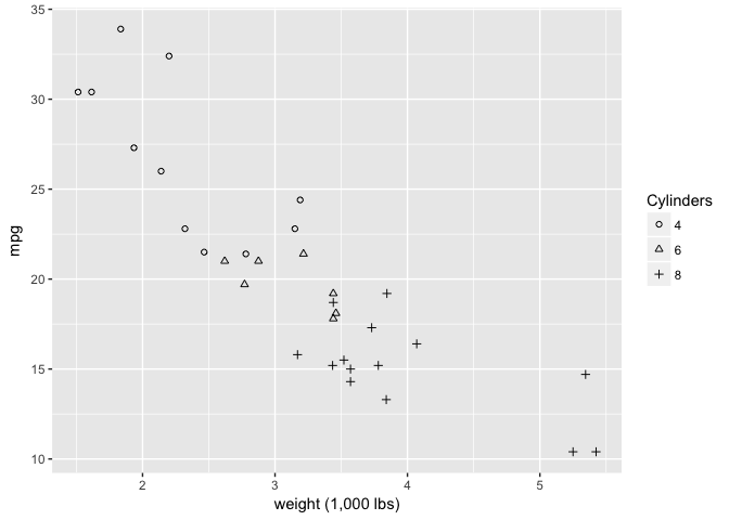
But these open ones are great.
ggplot(mtcars, aes(wt, mpg)) +
  geom_point(aes(shape=cyl), color="black") +
  xlab("weight (1,000 lbs)") +
  scale_shape_manual("Cylinders", values = c(1,2,3))
preso_save("img/wt_mpg_scatter_shape2.png")
It’s perfectly ok to redundantly encode using shape and color.
ggplot(mtcars, aes(wt, mpg)) +
  geom_point(aes(shape=cyl, color=cyl)) +
  xlab("weight (1,000 lbs)") +
  scale_shape_manual("Cylinders", values = c(1,2,3)) +
  scale_color_brewer("Cylinders", type="qual", palette=1)
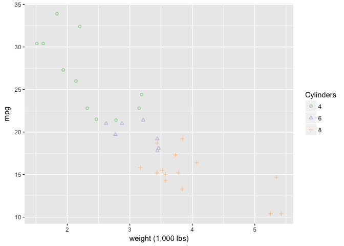
preso_save("img/wt_mpg_scatter_both.png")
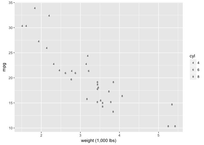
You’d think this would be a great encoding, but it’s terrible because of the similar curvature of the sixes and eights.
ggplot(mtcars, aes(wt, mpg)) +
  geom_point(aes(shape=cyl), color="black", size=2) +
  xlab("weight (1,000 lbs)") +
  scale_shape_manual(values = c(52,54,56))
preso_save("img/wt_mpg_scatter_letters.png")
Overlaying linear fits encloses space and makes the grouped objects very strong.
ggplot(mtcars, aes(wt, mpg)) +
  geom_point(aes(shape=cyl, color=cyl)) +
  geom_smooth(aes(group=cyl, color=cyl), method="lm") +
  xlab("weight (1,000 lbs)") +
  scale_shape_manual("Cylinders", values = c(1,2,3)) +
  scale_color_brewer("Cylinders", type="qual", palette=1)
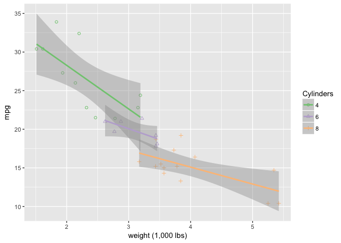
preso_save("img/wt_mpg_scatter_lm.png")
Law of Proximity
A dodged bar chart. Try to compare the blue vs. green bars. I find it very difficult.
ggplot(diamonds, aes(clarity, fill=cut, group=cut)) +
  geom_bar(stat="count", position="dodge") +
  scale_y_continuous("Count", labels=comma)
preso_save("img/diamonds_dodge.png")
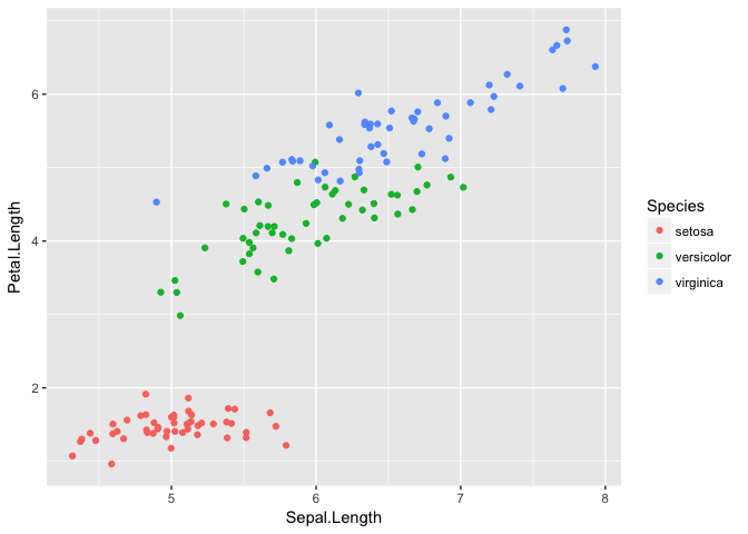
Assembly with iris data
Another dataset that’s good for demonstrating assembly. I didnt use these in the presentation.
ggplot(iris, aes(Sepal.Length, Sepal.Width, color=Species))+geom_jitter()
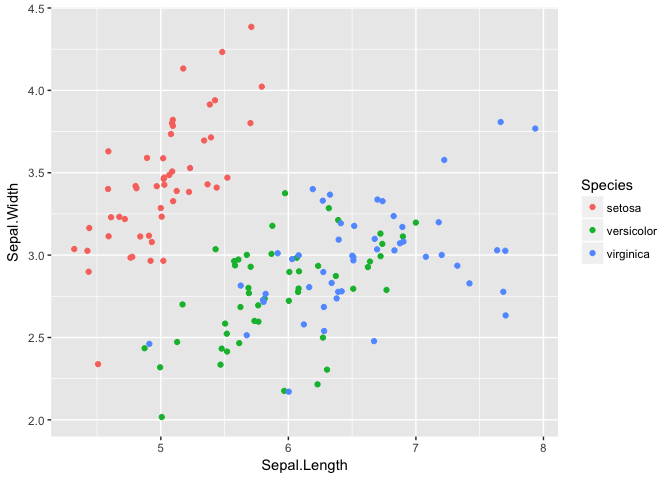
ggplot(iris, aes(Sepal.Length, Petal.Width, color=Species))+geom_jitter()
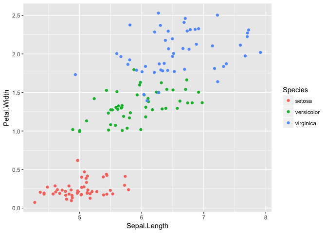
ggplot(iris, aes(Sepal.Length, Petal.Length, color=Species))+geom_jitter()
Part 4: Detection
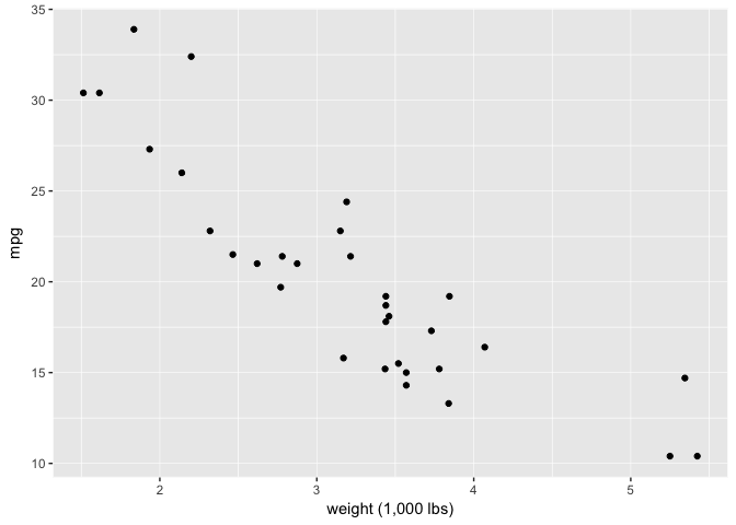
People frequenty hinder detection by lowering the contrast in luminance.
ggplot(mtcars, aes(wt, mpg)) +
  geom_point(color="gray30") +
  xlab("weight (1,000 lbs)")
preso_save("img/wt_mpg_scatter_grey.png")
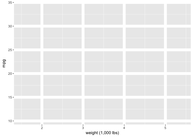
Or by hiding the data with non-data clutter, like gridlines.
ggplot(mtcars, aes(wt, mpg)) +
  geom_point(color="black", size=0.2) +
  xlab("weight (1,000 lbs)")

preso_save("img/wt_mpg_scatter_small.png")

theme_extras <- theme(panel.grid.major =   element_line(colour = "grey20", size = 0.2))
p<-ggplot(mtcars, aes(wt, mpg)) +
  geom_point(color="black", size=1.5) +
  xlab("weight (1,000 lbs)")

theme_extras <- theme(panel.border =       element_rect(fill = NA, colour = "white"),
                      panel.grid.major =   element_line(colour = "white", size = 0.2))
p+theme_extras
preso_save("img/wt_mpg_scatter_grid1.png", theme=theme_preso + theme_extras)

theme_extras <- theme(panel.border =       element_rect(fill = NA, colour = "white"),
                      panel.grid.minor =   element_line(colour = "white", size = 0.2),
                      panel.grid.major =   element_line(colour = "white", size = 0.5))
p+theme_extras

preso_save("img/wt_mpg_scatter_grid2.png", theme=theme_preso + theme_extras)

theme_extras <- theme(panel.border =       element_rect(fill = NA, colour = "white"),
                      panel.grid.minor =   element_line(colour = "white", size = 0.5),
                      panel.grid.major =   element_line(colour = "white", size = 1))
p+theme_extras

preso_save("img/wt_mpg_scatter_grid4.png", theme=theme_preso + theme_extras)
The Hermann Grid illusion. Do you see the faint grey dots?
theme_extras <- theme(panel.border =       element_rect(fill = NA, colour = "white"),
                      panel.grid.major =   element_line(colour = "white", size = 3.5))
ggplot(mtcars, aes(wt, mpg)) +
  geom_point(color="black", size=0, alpha=0) +
  xlab("weight (1,000 lbs)") + theme_extras
preso_save("img/wt_mpg_scatter_grid3.png", theme=theme_preso + theme_extras)
Decent grid and borders
theme_extras <- theme(panel.border =       element_rect(fill = NA, colour = "grey70"),
                      panel.grid.major =   element_line(colour = "grey70", size = 0.2))
p+theme_extras

preso_save("img/wt_mpg_scatter_grid5.png", theme=theme_preso + theme_extras)
Part 5: Other Useful results
Weber’s Law
weber <- data.frame(bar = c("c", "a", "b", "bb"),
                    zpad = c(3, 0, 0, 0),
                    ylen = c(10, 10.5, 0, 0),
                    xtop = c(2, 1.5, 0, 0))

weber1 <- weber %>%
  select(-xtop) %>%
  gather(var, val, -bar)

theme_extras <- theme(axis.title=element_blank(),
                      axis.text=element_blank(),
                      axis.ticks=element_blank(),
                      legend.position="none")
It’s hard to tell if the bars are the same legnth or different.
ggplot(weber1, aes(bar, val, fill=var)) + geom_bar(stat="identity") +
  scale_fill_manual(values=c("white", "black")) +
  expand_limits(y=c(0,15)) + theme_extras
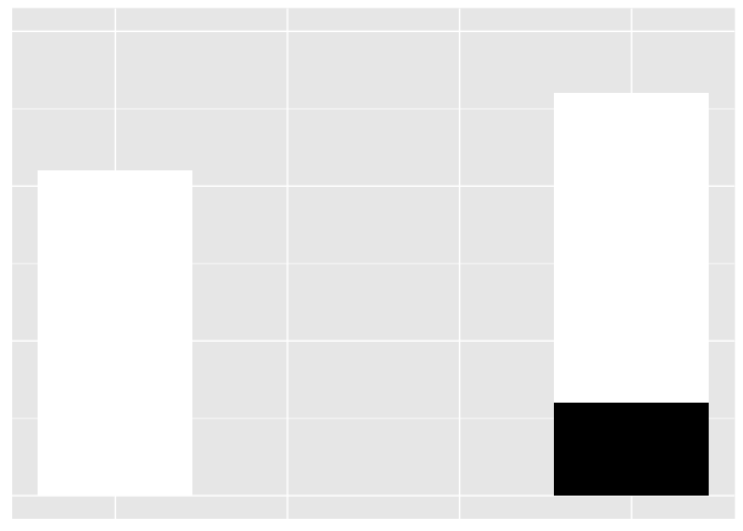
preso_save("img/weber1.png", theme=theme_preso+theme_extras)
But with the little blue ones, it’s easy, even though the absolute difference in length is exactly the same as with the white bars (0.5 units).
weber2 <- weber %>%
  gather(var, val, -bar)

ggplot(weber2, aes(bar, val, fill=var)) + geom_bar(stat="identity") +
  scale_fill_manual(values=c(muted("blue",l=60), "white", "black")) +
  expand_limits(y=c(0,15)) + theme_extras
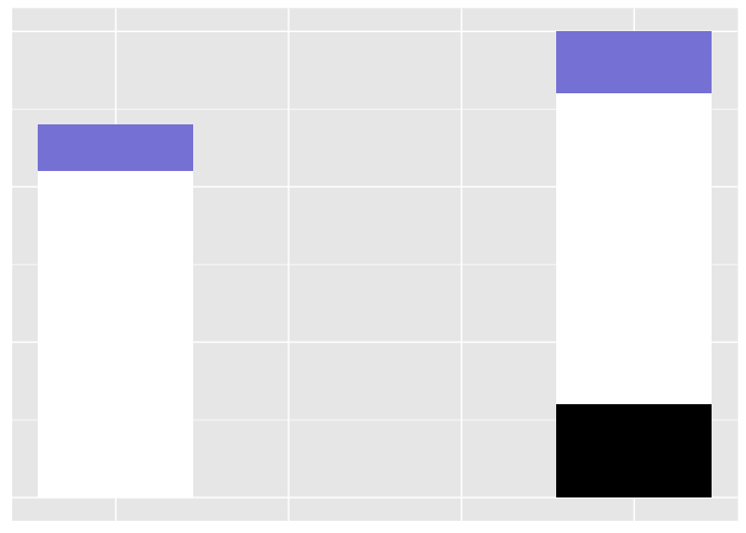
preso_save("img/weber2.png", theme=theme_preso+theme_extras)
Define eight different curves.
to_plot<-data.frame(x=seq(1,100,length.out=500)) %>%
  mutate(y=log(x),
         y2 = -(((x-100))^2),
         y03 = 100-1/x*y,
         y04 = 100-2/x*y,
         y05 = 100-2/(x+10)*y,
         y06 = 100-2/(x+5)*y,
         y07 = 99.8-1.5/(x+5)*y,
         y08 = 100-2.5/(x+5)*y,
         y09 = 100-1.5/(x+52)*y,
         y10 = 100-1.5/(x+25)*y
         )
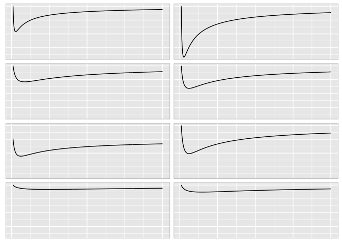
Without gridlines it’s hard to compare them precisely.
theme_extras <- theme(axis.title=element_blank(),
                      axis.text=element_blank(),
                      axis.ticks=element_blank(),
                      panel.border = element_rect(fill = NA, colour = "grey70"),
                      strip.text=element_blank())

ggplot(to_plot %>% select(-y2, -y) %>% gather(var, val, -x),
       aes(x,val)) + geom_line(color="black") + facet_wrap(~var, ncol=2) + theme_extras
preso_save("img/weber_grid1.png", width=1280/300/2, theme=theme_extras)
It’s much easier with gridlines, because of Weber’s law.
theme_extras <- theme(axis.title=element_blank(),
                      axis.text=element_blank(),
                      axis.ticks=element_blank(),
                      panel.border = element_rect(fill = NA, colour = "grey70"),
                      panel.grid.major = element_line(colour = "grey60", size = 0.2),
                      strip.text=element_blank())

ggplot(to_plot %>% select(-y2, -y) %>% gather(var, val, -x),
       aes(x,val)) + geom_line(color="black") + facet_wrap(~var, ncol=2) + theme_extras
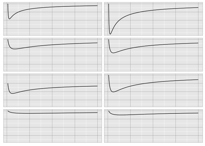
preso_save("img/weber_grid2.png", width=1280/300/2, theme=theme_extras)
You are most sensitive to changes in angle close to 45 degrees
The same data ploteed three ways. It’s easiest to detect the change in slope near 45 degrees.
dat<-data.frame(ct=c(1e6-10000, 1e6, 1e6+15000),
                dt=as.Date(c("2016-06-01","2016-06-02", "2016-06-03")))
p<-ggplot(dat, aes(dt, ct)) +
  geom_line(group=1, color="black") +
  geom_point(color="black") + ylab(NULL) + scale_x_date(NULL, labels=date_format("%b-%d"))
p
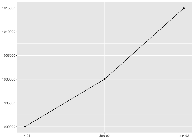
preso_save("img/45deg.png")
p + expand_limits(y=c(800000,1200000))
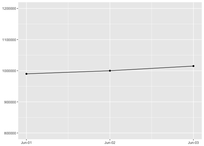
preso_save("img/45deg_tall.png")
p + expand_limits(x=as.Date(c("2016-05-01","2016-07-01")))
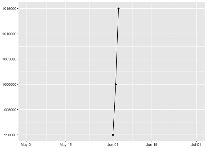
preso_save("img/45deg_wide.png")
Difficult to see with bars (where the y-axis must extend to zero).
ggplot(dat, aes(dt, ct)) +
  geom_bar(stat="identity", fill="white") +
  ylab(NULL) + scale_x_date(NULL, labels=date_format("%b-%d"))
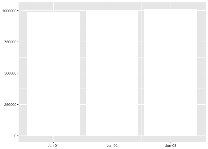
preso_save("img/45deg_bars.png", width=1280/300/2)
For banking to 45, see the example with the sunspots data in part 6.
The eye measures perdendicular distance
Where is the distance between the lines the greatest?
dat<-data.frame(x=seq(-10, 8, length.out = 100)) %>%
  mutate(y=-2*(x^2)+300,
         y2=y-seq(30,5,length.out = 100))

dat_w <- dat %>%
  gather(var, val, y, y2)

ggplot(dat_w, aes(x, val, group=var))+
  geom_line(color="black")
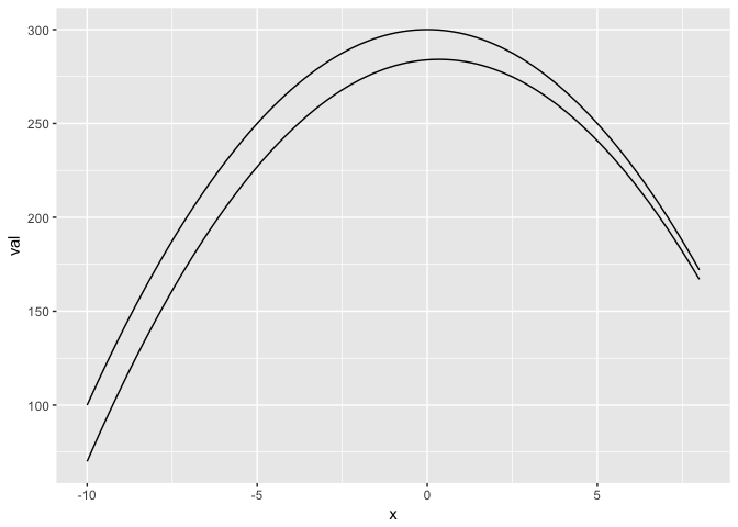
preso_save("img/gap_lines.png", width=1280/300*(2/3))
Here’s the distance plotted directly. Suprisingly, the distance is the largest at the left edge.
ggplot(dat, aes(x, y-y2)) + geom_line(color="black") + ylab("gap")
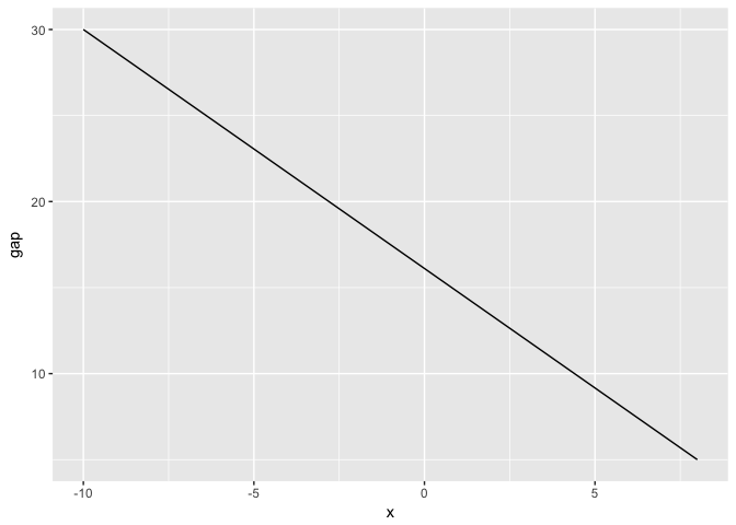
preso_save("img/gap_direct.png")
Y-axis to zero?
See the saturation, area and length examples from the estimation section with mtcars.
With bars the y-axis must go to zero. This obscures the variation in this dataset.
to_plot<-data.frame(x=1:20) %>%
  mutate(y=1e6 + 100*x*(-1)^x)
ggplot(to_plot, aes(x,y)) + geom_bar(fill="white",stat="identity") + xlab(NULL) + ylab(NULL)
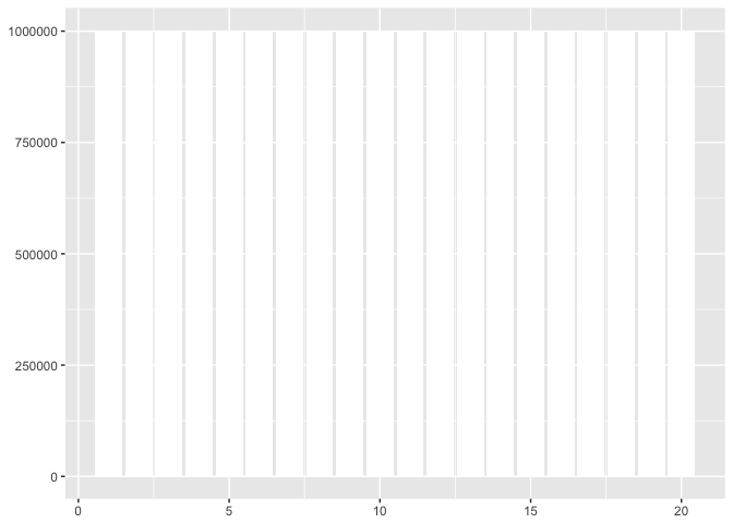
preso_save("img/yaxis_bars.png")
If we switch to points (and position on a common scale), we are free to clip the y-axis to just the relevant interval.
ggplot(to_plot, aes(x,y)) + geom_line(color="black") + geom_point(color="black") + xlab(NULL) + ylab(NULL)
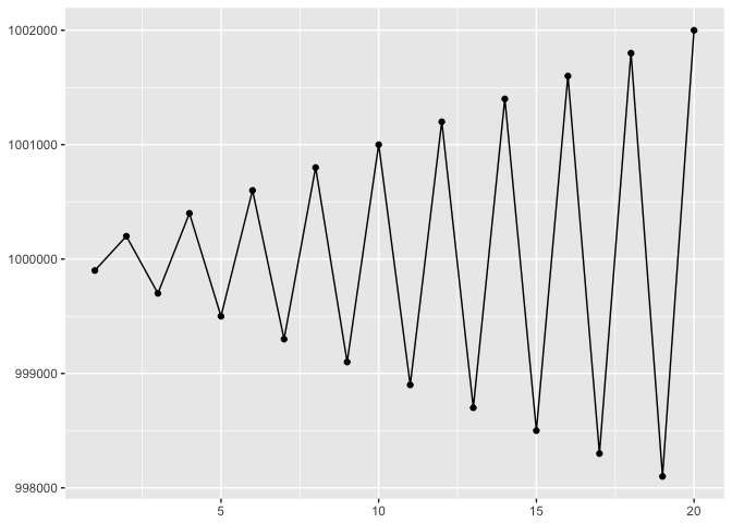
preso_save("img/yaxis_lines.png")
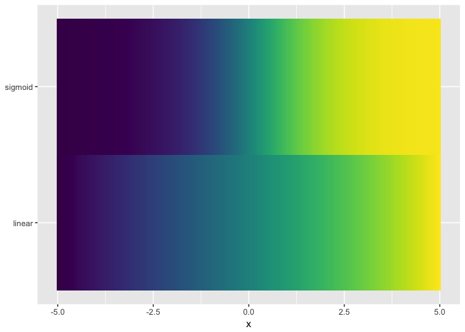
Hue (used carefully) is good for revealing fine structure
ramps<-data.frame(x=seq(-5,5,length.out=200)) %>%
  mutate(linear=x/10+0.5,
         sigmoid=1/(1+exp(-x)))

theme_extras <- theme(axis.title.y=element_blank(),
                      axis.text.y=element_blank(),
                      axis.ticks.y=element_blank(),
                      legend.position="none")

ggplot(ramps, aes(x,1,fill=sigmoid)) + geom_tile() + theme_extras
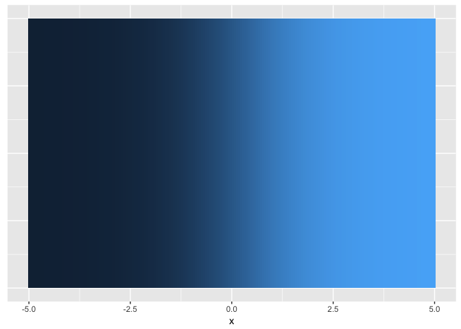
preso_save("img/ramp_sigmoid.png", theme=theme_preso+theme_extras)

ggplot(ramps, aes(x,1,fill=linear)) + geom_tile() + theme_extras
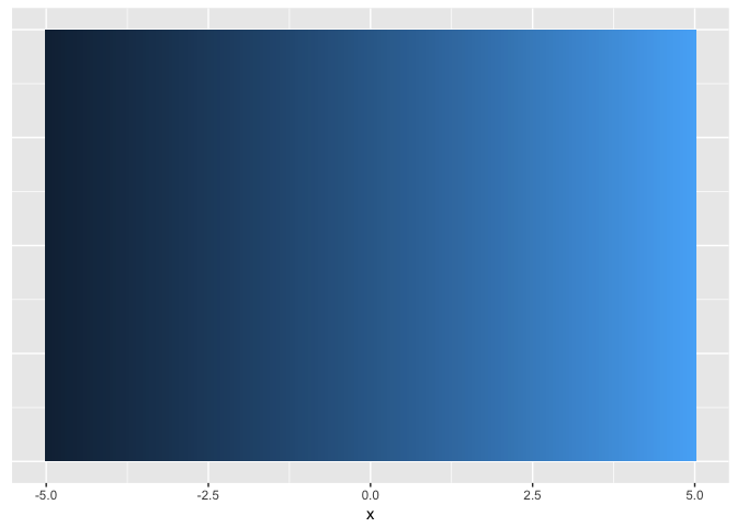
preso_save("img/ramp_linear.png", theme=theme_preso+theme_extras)

theme_extras <- theme(axis.title.y=element_blank(),
                      axis.text.y=element_blank(),
                      axis.ticks.y=element_blank())

ggplot(ramps %>% gather(series,value,-x), aes(x,value,color=series)) + geom_line() + theme_extras
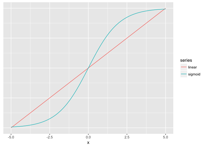
preso_save("img/ramp_both_lines.png", theme=theme_preso+theme_extras)

theme_extras <- theme(axis.title.y=element_blank(),
                      legend.position="none")

ggplot(ramps %>% gather(series,value,-x), aes(x,series,fill=value)) + geom_tile() + theme_extras
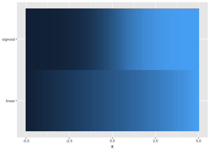
preso_save("img/ramp_both.png", theme=theme_preso+theme_extras)

jet.colors <- colorRampPalette(c("#00007F", "blue", "#007FFF", "cyan", "#7FFF7F", "yellow", "#FF7F00", "red", "#7F0000"))
ggplot(ramps %>% gather(series,value,-x), aes(x,series,fill=value)) + geom_tile() + theme_extras + scale_fill_gradientn(colors = jet.colors(7))
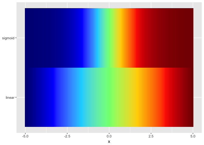
preso_save("img/ramp_both_hue.png", theme=theme_preso+theme_extras)
Viridis not a good as colorjet. Presumably because colorjet traverses more of the space of colors.
ggplot(ramps %>% gather(series,value,-x), aes(x,series,fill=value)) + geom_tile() + theme_extras + scale_fill_viridis()
Part 6: Tools/Workflow
Sunspot data
The data is from: http://www.sidc.be/silso/DATA/SN_d_tot_V2.0.txt.
First we load it in and tidy it up.
# Format:
#Line format [character position]:
#- [1-4] Year
#- [6-7] Month
#- [9-10] Day
#- [12-19] Decimal date
#- [22-24] Daily sunspot number
#- [26-30] Standard deviation
#- [33-35] Number of observations
#- [37] Definitive/provisional indicator

positions <- fwf_positions(start=c(1,6,9,12,22,26,33,37),
                           end=c(4,7,10,19,24,30,35,37),
                           col_names=c("year", "month", "day", "decimal_date",
                                       "sunspot_number", "std_dev", "n", "provisional"))
sunspots_raw<-read_fwf("http://www.sidc.be/silso/DATA/SN_d_tot_V2.0.txt", col_positions=positions)
## Parsed with column specification:
## cols(
##   year = col_integer(),
##   month = col_integer(),
##   day = col_character(),
##   decimal_date = col_double(),
##   sunspot_number = col_integer(),
##   std_dev = col_double(),
##   n = col_integer(),
##   provisional = col_character()
## )
sunspots <- sunspots_raw %>%
  mutate(day = as.integer(day),
         dt = as.Date(sprintf("%4d-%02d-%02d", year, month, day)),
         sunspot_number = ifelse(sunspot_number==-1, NA, as.numeric(sunspot_number)),
         std_dev = ifelse(std_dev==-1, NA, std_dev),
         provisional = !is.na(provisional)) %>%
  # There are many missing values before 1850 which complicate analysis
  filter(dt >= "1850-01-01") %>%
  select(-year, -month, -day, -decimal_date)
summary(sunspots)
##  sunspot_number      std_dev             n          provisional
##  Min.   :  0.00   Min.   : 0.000   Min.   : 1.000   Mode :logical
##  1st Qu.: 22.00   1st Qu.: 3.600   1st Qu.: 1.000   FALSE:61177
##  Median : 65.00   Median : 6.700   Median : 1.000   TRUE :92
##  Mean   : 84.89   Mean   : 7.075   Mean   : 4.765
##  3rd Qu.:130.00   3rd Qu.: 9.900   3rd Qu.: 1.000
##  Max.   :528.00   Max.   :77.700   Max.   :58.000
##        dt
##  Min.   :1850-01-01
##  1st Qu.:1891-12-09
##  Median :1933-11-16
##  Mean   :1933-11-16
##  3rd Qu.:1975-10-24
##  Max.   :2017-09-30
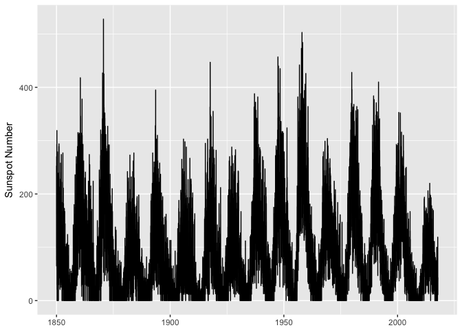
A first attempt at plotting… yuck.
ggplot(sunspots, aes(dt, sunspot_number)) +
  geom_line(color="black") +
  xlab(NULL) + ylab("Sunspot Number")
preso_save("img/sunspots_line.png")
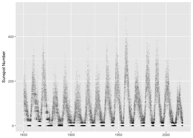
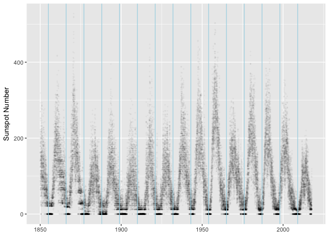
Plot as dots, use alpha transparency to reduce overplotting. Notice the gaps between zero and non-zero. You wouldn’t have noticed those without visualization.
ggplot(sunspots, aes(dt, sunspot_number)) +
  geom_point(size=0.5, alpha=1/40, color="black") +
  xlab(NULL) + ylab("Sunspot Number")
preso_save("img/sunspots_point.png")
There are lots of things we could try to explain about this data, but the most obivous one is the major cycle that’s about 11 years long.
minima <- as.Date("1954-01-01") + seq(-9, 5) * 11 * 365.25
ggplot(sunspots, aes(dt, sunspot_number)) +
  geom_point(size=0.5, alpha=1/40, color="black") +
  geom_vline(xintercept=as.numeric(minima), color="lightblue") +
  xlab(NULL) + ylab("Sunspot Number")
preso_save("img/sunspots_vlines.png")
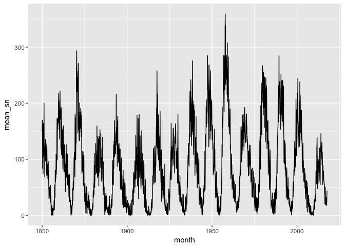
To make it easier to work with, let’s take monthly averages of the data.
# This works, but it's silly to work on this data at a daily level
#sunspots_ts<- ts(sunspots$sunspot_number, frequency=11*365.25)
#z <- fourier(sunspots_ts, K=3)
#fit <- auto.arima(sunspots_ts, d=1, xreg=z, allowdrift = F, seasonal=FALSE, trace = T)

sunspots_month <- sunspots %>%
  mutate(month = as.Date(format(dt, "%Y-%m-01"))) %>%
  group_by(month) %>%
  summarize(mean_sn = mean(sunspot_number, na.rm=T))
summary(sunspots_month)
##      month               mean_sn
##  Min.   :1850-01-01   Min.   :  0.00
##  1st Qu.:1891-12-01   1st Qu.: 25.90
##  Median :1933-11-01   Median : 72.55
##  Mean   :1933-10-31   Mean   : 84.89
##  3rd Qu.:1975-10-01   3rd Qu.:127.79
##  Max.   :2017-09-01   Max.   :359.39
ggplot(sunspots_month, aes(month, mean_sn)) + geom_line(color="black")
preso_save("img/sunspots_month.png")
#ggplot(sunspots_month, aes(month, mean_sn)) + geom_point(color="black")
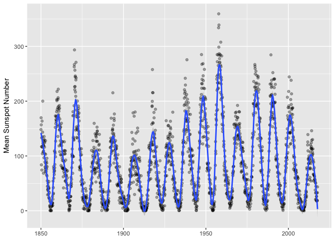
Now we can put a loess smoother over the monthly data, and we finally have a nice visualization of the series.
ggplot(sunspots_month, aes(month, mean_sn)) + geom_point(color="black", alpha=1/3) +
  geom_smooth(method="loess", span=0.05, n=400) +
  xlab(NULL) + ylab("Mean Sunspot Number")
preso_save("img/sunspots_month_smooth.png")
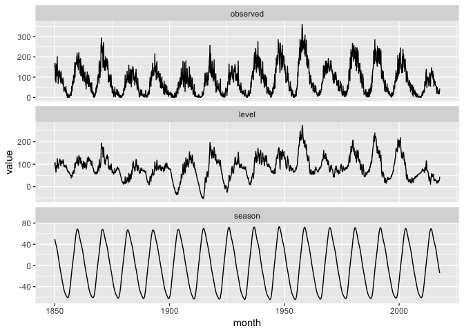
Now let’s impose a model on the data.
library(forecast)
## Warning: package 'forecast' was built under R version 3.4.2
tb<-tbats(sunspots_month$mean_sn,
          use.trend=F, use.box.cox=F,
          seasonal.periods = c(12*11))
tb_components_mat<-tbats.components(tb)
tb_components<-data.frame(month=sunspots_month$month,
                          observed = tb_components_mat[,"observed"],
                          level = tb_components_mat[,"level"],
                          season = tb_components_mat[,"season"],
                          residuals = residuals(tb),
                          fitted = fitted(tb))

tb_components_w <- tb_components %>%
  gather(variable, value, -month) %>%
  mutate(variable = factor(variable, levels=c("observed", "level", "season", "fitted", "residuals")))
… and visualize the results of the model.
ggplot(tb_components_w %>% filter(variable %in% c("observed","level","season")),
       aes(month, value)) +
  geom_line(color="black") +
  facet_wrap(~variable, ncol=1, scales="free_y")
preso_save("img/sunspots_tbats.png")
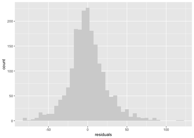
But is the model good? A common model diagnostic is to look at the “residuals” the difference between the observed data and the model. According to our model, this should be normally distributed with a mean of zero.
binw=5
ggplot(tb_components, aes(residuals)) + geom_histogram(binwidth=binw, fill="lightgrey")
preso_save("img/sunspots_residuals.png")
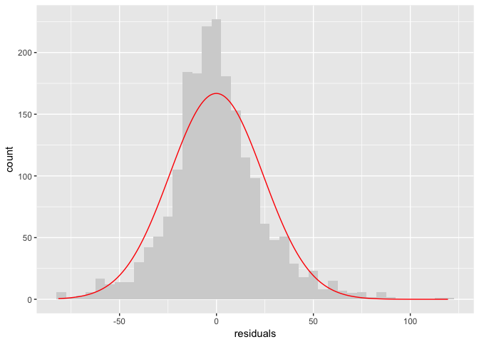
If you don’t have great intuition about what a normal curve looks like, it can help to overlay one. It look like our model ok, but not great.
curve = data.frame(x=seq(min(tb_components$residuals), max(tb_components$residuals), length.out = 200)) %>%
  mutate(y=(binw*length(tb_components$residuals)) * dnorm(x, mean(tb_components$residuals), sd(tb_components$residuals)))
ggplot(tb_components, aes(residuals)) + geom_histogram(binwidth=binw, fill="lightgrey") +
  geom_line(data=curve, aes(x,y), color="red")
# Other diagnostic plots
qqnorm(residuals(tb))
plot(acf(residuals(tb), lag.max=150))
# 11 year moving average
plot(ma(sunspots$sunspot_number, round(365.25*11)))
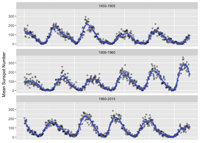
Demonstrates banking to 45. There seems to be a pattern of a sharper attack and slower decay.
sunspots_month <- sunspots_month %>%
#  mutate(piece = ifelse(month < '1900-01-01', "1850-1900", ifelse(month < '1950-01-01', "1900-1950", "1950-2000"))) %>%
  mutate(piece = ifelse(month < '1905-01-01', "1850-1905", ifelse(month < '1960-01-01', "1906-1960", "1960-2015"))) %>%
  group_by(piece) %>%
  mutate(obs=1:length(month)) %>%
  ungroup()

theme_extras <- theme(axis.title.x=element_blank(),
                      axis.text.x=element_blank(),
                      axis.ticks.x=element_blank())

ggplot(sunspots_month %>% filter(month < '2015-01-01'),
       aes(obs, mean_sn)) + geom_point(color="black", alpha=1/3) +
  geom_smooth(method="loess", span=0.05*2, n=150) + facet_wrap(~piece, ncol=1) +
  theme_extras +
  ylab("Mean Sunspot Number")
preso_save("img/sunspots_month_wide.png", theme=theme_preso + theme_extras)
Appendix
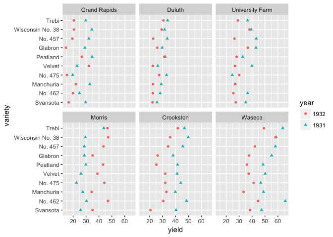
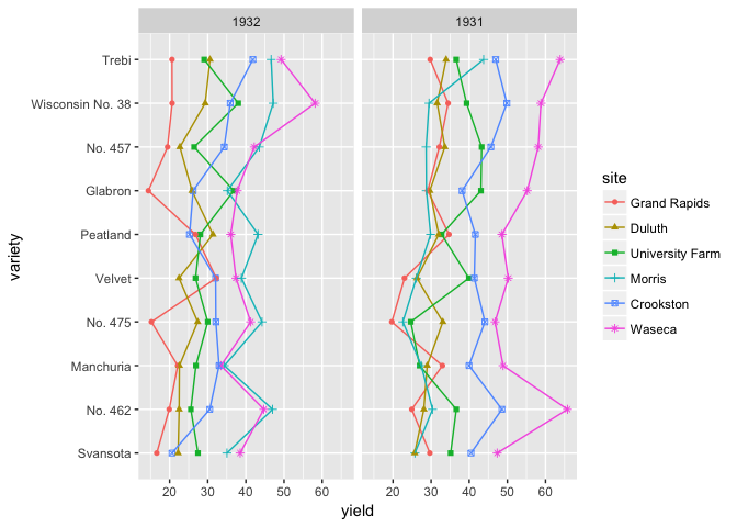
Barley dataset
library(lattice) # For the barley dataset
# If you want to encourage comparing between years, then put them on a common scale
ggplot(barley, aes(yield, variety, color=year, shape=year))+
  geom_point()+facet_wrap(~site)
# If you want to encourage comparing between sites, then put them on a common scale
ggplot(barley, aes(variety, yield, group=site, color=site, shape=site))+
  geom_point()+geom_line()+facet_wrap(~year)+coord_flip()
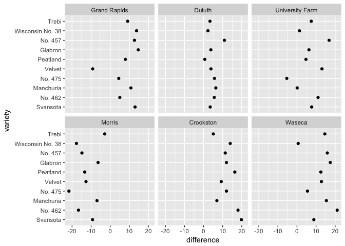
# Can you spot the anomaly?
barley_differences <- barley %>%
  group_by(variety, site) %>%
  arrange(year) %>%
  summarize(difference = yield[2]-yield[1])

ggplot(barley_differences,
       aes(difference, variety))+
  geom_point(color="black") + facet_wrap(~site)
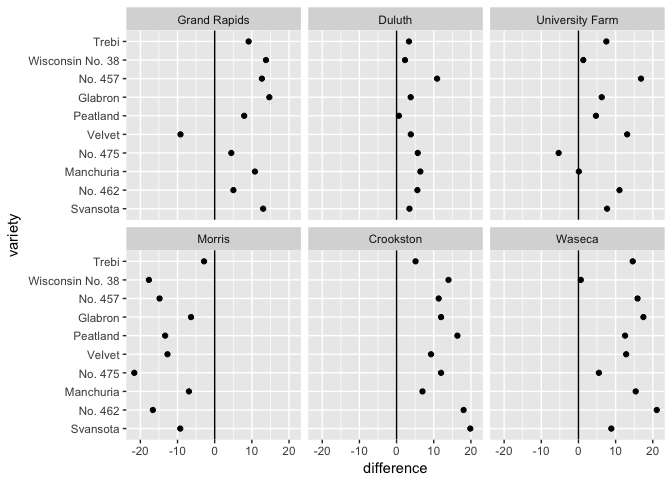
ggplot(barley_differences,
       aes(difference, variety))+
  geom_point(color="black") + geom_vline(xintercept=0) + facet_wrap(~site)
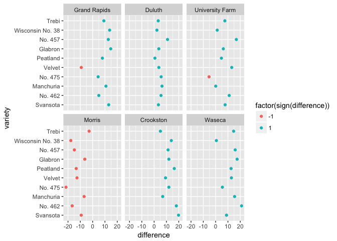
ggplot(barley_differences,
       aes(difference, variety, color=factor(sign(difference))))+
  geom_point()+facet_wrap(~site)
Session Information
sessionInfo()
## R version 3.4.1 (2017-06-30)
## Platform: x86_64-apple-darwin15.6.0 (64-bit)
## Running under: macOS Sierra 10.12.6
##
## Matrix products: default
## BLAS: /Library/Frameworks/R.framework/Versions/3.4/Resources/lib/libRblas.0.dylib
## LAPACK: /Library/Frameworks/R.framework/Versions/3.4/Resources/lib/libRlapack.dylib
##
## locale:
## [1] en_US.UTF-8/en_US.UTF-8/en_US.UTF-8/C/en_US.UTF-8/en_US.UTF-8
##
## attached base packages:
## [1] stats     graphics  grDevices utils     datasets  methods   base
##
## other attached packages:
##  [1] lattice_0.20-35   bindrcpp_0.2      gapminder_0.2.0
##  [4] viridis_0.4.0     viridisLite_0.2.0 broom_0.4.2
##  [7] scales_0.5.0      stringr_1.2.0     tidyr_0.7.1
## [10] dplyr_0.7.4       readr_1.1.1       ggplot2_2.2.1
##
## loaded via a namespace (and not attached):
##  [1] Rcpp_0.12.13       RColorBrewer_1.1-2 compiler_3.4.1
##  [4] plyr_1.8.4         bindr_0.1          tools_3.4.1
##  [7] digest_0.6.12      evaluate_0.10.1    tibble_1.3.4
## [10] gtable_0.2.0       nlme_3.1-131       pkgconfig_2.0.1
## [13] rlang_0.1.2        psych_1.7.8        curl_2.8.1
## [16] yaml_2.1.14        parallel_3.4.1     gridExtra_2.3
## [19] knitr_1.17         hms_0.3            tidyselect_0.2.0
## [22] rprojroot_1.2      grid_3.4.1         glue_1.1.1
## [25] R6_2.2.2           foreign_0.8-69     rmarkdown_1.6
## [28] reshape2_1.4.2     purrr_0.2.3        magrittr_1.5
## [31] backports_1.1.1    htmltools_0.3.6    assertthat_0.2.0
## [34] mnormt_1.5-5       colorspace_1.3-2   labeling_0.3
## [37] stringi_1.1.5      lazyeval_0.2.0     munsell_0.4.3