BGGN-213, Lecture 18
Pathway analysis from RNA-seq differential expression results
Overview
Analysis of high-throughput biological data typically yields a list of genes or proteins requiring further interpretation - for example the ranked lists of differentially expressed genes we have been generating from our RNA-seq analysis to date.
Our intention is typically to use such lists to gain novel insights about genes and proteins that may have roles in a given phenomenon, phenotype or disease progression. However, in many cases these ‘raw’ gene lists are challenging to interpret due to their large size and lack of useful annotations. Hence, our expensively assembled gene lists often fail to convey the full degree of possible insight about the condition being studied.
Pathway analysis (also known as gene set analysis or over-representation analysis), aims to reduce the complexity of interpreting gene lists via mapping the listed genes to known (i.e. annotated) biological pathways, processes and functions.
Side-note: Pathway analysis can actually mean many different things to different people. This includes analysis of Gene Ontology (GO) terms, protein–protein interaction networks, flux-balance analysis from kinetic simulations of pathways, etc. However, pathway analysis most commonly focuses on methods that exploit existing pathway knowledge (e.g. in public repositories such as GO or KEGG), rather than on methods that infer pathways from molecular measurements. These more general approaches are nicely reviewed in this paper:
- Khatri, et al. “Ten years of pathway analysis: current approaches and outstanding challenges.” PLoS Comput Biol 8.2 (2012): e1002375.
Patway analysis with R and Bioconductor
There are many freely available tools for pathway or over-representation analysis. As of Nov 2017 Bioconductor alone has over 80 packages categorized under gene set enrichment and over 120 packages categorized under pathways.
Here we play with just one, the GAGE package (which stands for Generally Applicable Gene set Enrichment), to do KEGG pathway enrichment analysis on RNA-seq based differential expression results.
The KEGG pathway database, unlike GO for example, provides functional annotation as well as information about gene products that interact with each other in a given pathway, how they interact (e.g., activation, inhibition, etc.), and where they interact (e.g., cytoplasm, nucleus, etc.). Hence KEGG has the potential to provide extra insight beyond annotation lists of simple molecular function, process etc. from GO terms.
In this analysis, we check for coordinated differential expression over gene sets from KEGG pathways instead of changes of individual genes. The assumption here is that consistent perturbations over a given pathway (gene set) may suggest mechanistic changes.
About our Input Data
The data for for hands-on session comes from GEO entry: GSE37704, which is associated with the following publication:
- Trapnell C, Hendrickson DG, Sauvageau M, Goff L et al. “Differential analysis of gene regulation at transcript resolution with RNA-seq”. Nat Biotechnol 2013 Jan;31(1):46-53. PMID: 23222703
The authors report on differential analysis of lung fibroblasts in response to loss of the developmental transcription factor HOXA1. Their results and others indicate that HOXA1 is required for lung fibroblast and HeLa cell cycle progression. In particular their analysis show that “loss of HOXA1 results in significant expression level changes in thousands of individual transcripts, along with isoform switching events in key regulators of the cell cycle”. For our session we have used their Sailfish gene-level estimated counts and hence are restricted to protein-coding genes only.
Section 1. Differential Expression Analysis
You can download the count data and associated metadata from here: GSE37704_featurecounts.csv and GSE37704_metadata.csv. This is similar to our starting point for the last class where we used DESeq2 for the first time. We will use it again today!
#library(dplyr)
library(DESeq2)
Load our data files
metaFile <- "data/GSE37704_metadata.csv"
countFile <- "data/GSE37704_featurecounts.csv"

# Import metadata and take a peak
colData = read.csv(metaFile, row.names=1)
head(colData)
##               condition
## SRR493366 control_sirna
## SRR493367 control_sirna
## SRR493368 control_sirna
## SRR493369      hoxa1_kd
## SRR493370      hoxa1_kd
## SRR493371      hoxa1_kd
# Import countdata
countData = read.csv(countFile, row.names=1)
head(countData)
##                 length SRR493366 SRR493367 SRR493368 SRR493369 SRR493370
## ENSG00000186092    918         0         0         0         0         0
## ENSG00000279928    718         0         0         0         0         0
## ENSG00000279457   1982        23        28        29        29        28
## ENSG00000278566    939         0         0         0         0         0
## ENSG00000273547    939         0         0         0         0         0
## ENSG00000187634   3214       124       123       205       207       212
##                 SRR493371
## ENSG00000186092         0
## ENSG00000279928         0
## ENSG00000279457        46
## ENSG00000278566         0
## ENSG00000273547         0
## ENSG00000187634       258
Hmm… remember that we need the countData and colData files to match up so we will need to remove that odd first column in countData namely contData$length.
# Note we need to remove the odd first $length col
countData <- as.matrix(countData[,-1])
head(countData)
##                 SRR493366 SRR493367 SRR493368 SRR493369 SRR493370
## ENSG00000186092         0         0         0         0         0
## ENSG00000279928         0         0         0         0         0
## ENSG00000279457        23        28        29        29        28
## ENSG00000278566         0         0         0         0         0
## ENSG00000273547         0         0         0         0         0
## ENSG00000187634       124       123       205       207       212
##                 SRR493371
## ENSG00000186092         0
## ENSG00000279928         0
## ENSG00000279457        46
## ENSG00000278566         0
## ENSG00000273547         0
## ENSG00000187634       258
This looks better but there are lots of zero entries in there so let’s get rid of them as we have no data for these.
# Filter count data where you have 0 read count across all samples.
countData = countData[rowSums(countData)>1, ]
head(countData)
##                 SRR493366 SRR493367 SRR493368 SRR493369 SRR493370
## ENSG00000279457        23        28        29        29        28
## ENSG00000187634       124       123       205       207       212
## ENSG00000188976      1637      1831      2383      1226      1326
## ENSG00000187961       120       153       180       236       255
## ENSG00000187583        24        48        65        44        48
## ENSG00000187642         4         9        16        14        16
##                 SRR493371
## ENSG00000279457        46
## ENSG00000187634       258
## ENSG00000188976      1504
## ENSG00000187961       357
## ENSG00000187583        64
## ENSG00000187642        16
Nice now lets setup the DESeqDataSet object required for the DESeq() function and then run the DESeq pipeline. This is again similar to our last days hands-on session.
dds = DESeqDataSetFromMatrix(countData=countData,
                             colData=colData,
                             design=~condition)
dds = DESeq(dds)
## estimating size factors

## estimating dispersions

## gene-wise dispersion estimates

## mean-dispersion relationship

## final dispersion estimates

## fitting model and testing
dds
## class: DESeqDataSet
## dim: 15280 6
## metadata(1): version
## assays(3): counts mu cooks
## rownames(15280): ENSG00000279457 ENSG00000187634 ...
##   ENSG00000276345 ENSG00000271254
## rowData names(21): baseMean baseVar ... deviance maxCooks
## colnames(6): SRR493366 SRR493367 ... SRR493370 SRR493371
## colData names(2): condition sizeFactor
Next, get results for the HoxA1 knockdown versus control siRNA (remember we labeled these as “hoxa1_kd” and “control_sirna” in our original colData metaFile input to DESeq, you can check this above and by running resultsNames(dds) command).
res = results(dds, contrast=c("condition", "hoxa1_kd", "control_sirna"))
Let’s reorder these results by p-value and call summary() on the results object to get a sense of how many genes are up or down-regulated at the default FDR of 0.1.
res = res[order(res$pvalue),]
summary(res)
##
## out of 15280 with nonzero total read count
## adjusted p-value < 0.1
## LFC > 0 (up)     : 4352, 28%
## LFC < 0 (down)   : 4400, 29%
## outliers [1]     : 0, 0%
## low counts [2]   : 590, 3.9%
## (mean count < 1)
## [1] see 'cooksCutoff' argument of ?results
## [2] see 'independentFiltering' argument of ?results
Since we mapped and counted against the Ensembl annotation, our results only have information about Ensembl gene IDs. However, our pathway analysis downstream will use KEGG pathways, and genes in KEGG pathways are annotated with Entrez gene IDs. So lets add them as we did the last day.
library("AnnotationDbi")
library("org.Hs.eg.db")

columns(org.Hs.eg.db)
##  [1] "ACCNUM"       "ALIAS"        "ENSEMBL"      "ENSEMBLPROT"
##  [5] "ENSEMBLTRANS" "ENTREZID"     "ENZYME"       "EVIDENCE"
##  [9] "EVIDENCEALL"  "GENENAME"     "GO"           "GOALL"
## [13] "IPI"          "MAP"          "OMIM"         "ONTOLOGY"
## [17] "ONTOLOGYALL"  "PATH"         "PFAM"         "PMID"
## [21] "PROSITE"      "REFSEQ"       "SYMBOL"       "UCSCKG"
## [25] "UNIGENE"      "UNIPROT"
res$symbol = mapIds(org.Hs.eg.db,
                    keys=row.names(res),
                    column="SYMBOL",
                    keytype="ENSEMBL",
                    multiVals="first")

res$entrez = mapIds(org.Hs.eg.db,
                    keys=row.names(res),
                    column="ENTREZID",
                    keytype="ENSEMBL",
                    multiVals="first")

res$name =   mapIds(org.Hs.eg.db,
                    keys=row.names(res),
                    column="GENENAME",
                    keytype="ENSEMBL",
                    multiVals="first")

head(res, 10)
## log2 fold change (MLE): condition hoxa1_kd vs control_sirna
## Wald test p-value: condition hoxa1 kd vs control sirna
## DataFrame with 10 rows and 9 columns
##                  baseMean log2FoldChange      lfcSE      stat    pvalue
##                 <numeric>      <numeric>  <numeric> <numeric> <numeric>
## ENSG00000117519  4483.627      -2.422719 0.06001850 -40.36620         0
## ENSG00000183508  2053.881       3.201955 0.07241968  44.21388         0
## ENSG00000159176  5692.463      -2.313737 0.05757255 -40.18820         0
## ENSG00000150938  7442.986      -2.059631 0.05386627 -38.23601         0
## ENSG00000116016  4423.947      -1.888019 0.04318301 -43.72134         0
## ENSG00000136068  3796.127      -1.649792 0.04394825 -37.53942         0
## ENSG00000164251  2348.770       3.344508 0.06907610  48.41773         0
## ENSG00000124766  2576.653       2.392288 0.06171493  38.76352         0
## ENSG00000124762 28106.119       1.832258 0.03892405  47.07264         0
## ENSG00000106366 43719.126      -1.844046 0.04194432 -43.96415         0
##                      padj      symbol      entrez
##                 <numeric> <character> <character>
## ENSG00000117519         0        CNN3        1266
## ENSG00000183508         0      FAM46C       54855
## ENSG00000159176         0       CSRP1        1465
## ENSG00000150938         0       CRIM1       51232
## ENSG00000116016         0       EPAS1        2034
## ENSG00000136068         0        FLNB        2317
## ENSG00000164251         0       F2RL1        2150
## ENSG00000124766         0        SOX4        6659
## ENSG00000124762         0      CDKN1A        1026
## ENSG00000106366         0    SERPINE1        5054
##                                                        name
##                                                 <character>
## ENSG00000117519                                  calponin 3
## ENSG00000183508 family with sequence similarity 46 member C
## ENSG00000159176         cysteine and glycine rich protein 1
## ENSG00000150938 cysteine rich transmembrane BMP regulator 1
## ENSG00000116016            endothelial PAS domain protein 1
## ENSG00000136068                                   filamin B
## ENSG00000164251                 F2R like trypsin receptor 1
## ENSG00000124766                                   SRY-box 4
## ENSG00000124762        cyclin dependent kinase inhibitor 1A
## ENSG00000106366                    serpin family E member 1
Great, this is looking good so far. Now lets see how pathway analysis can help us make further sense out of this ranked list of differentially expressed genes.
Section 2. Pathway Analysis
Here we are going to use the gage package for pathway analysis. Once we have a list of enriched pathways, we’re going to use the pathview package to draw pathway diagrams, shading the molecules in the pathway by their degree of up/down-regulation.
KEGG pathways
The gageData package has pre-compiled databases mapping genes to KEGG pathways and GO terms for common organisms. kegg.sets.hs is a named list of 229 elements. Each element is a character vector of member gene Entrez IDs for a single KEGG pathway. (See also go.sets.hs). The sigmet.idx.hs is an index of numbers of signaling and metabolic pathways in kegg.set.gs. In other words, KEGG pathway include other types of pathway definitions, like “Global Map” and “Human Diseases”, which may be undesirable in pathway analysis. Therefore, kegg.sets.hs[sigmet.idx.hs] gives you the “cleaner” gene sets of signaling and metabolic pathways only.
Side-Note: While there are many freely available tools to do pathway analysis, and some like gage are truly fantastic, many of them are poorly maintained or rarely updated. The DAVID tool that a lot of folks use for simple gene set enrichment analysis was not updated at all between Jan 2010 and Oct 2016.
First we need to do our one time install of these required bioconductor packages:
source("http://bioconductor.org/biocLite.R")
biocLite( c("pathview", "gage", "gageData") )
Now we can load the packages and setup the KEGG data-sets we need.
library(pathview)
## ##############################################################################
## Pathview is an open source software package distributed under GNU General
## Public License version 3 (GPLv3). Details of GPLv3 is available at
## http://www.gnu.org/licenses/gpl-3.0.html. Particullary, users are required to
## formally cite the original Pathview paper (not just mention it) in publications
## or products. For details, do citation("pathview") within R.
##
## The pathview downloads and uses KEGG data. Non-academic uses may require a KEGG
## license agreement (details at http://www.kegg.jp/kegg/legal.html).
## ##############################################################################
library(gage)
library(gageData)

data(kegg.sets.hs)
data(sigmet.idx.hs)

kegg.sets.hs = kegg.sets.hs[sigmet.idx.hs]
head(kegg.sets.hs, 3)
## $`hsa00232 Caffeine metabolism`
## [1] "10"   "1544" "1548" "1549" "1553" "7498" "9"
##
## $`hsa00983 Drug metabolism - other enzymes`
##  [1] "10"     "1066"   "10720"  "10941"  "151531" "1548"   "1549"
##  [8] "1551"   "1553"   "1576"   "1577"   "1806"   "1807"   "1890"
## [15] "221223" "2990"   "3251"   "3614"   "3615"   "3704"   "51733"
## [22] "54490"  "54575"  "54576"  "54577"  "54578"  "54579"  "54600"
## [29] "54657"  "54658"  "54659"  "54963"  "574537" "64816"  "7083"
## [36] "7084"   "7172"   "7363"   "7364"   "7365"   "7366"   "7367"
## [43] "7371"   "7372"   "7378"   "7498"   "79799"  "83549"  "8824"
## [50] "8833"   "9"      "978"
##
## $`hsa00230 Purine metabolism`
##   [1] "100"    "10201"  "10606"  "10621"  "10622"  "10623"  "107"
##   [8] "10714"  "108"    "10846"  "109"    "111"    "11128"  "11164"
##  [15] "112"    "113"    "114"    "115"    "122481" "122622" "124583"
##  [22] "132"    "158"    "159"    "1633"   "171568" "1716"   "196883"
##  [29] "203"    "204"    "205"    "221823" "2272"   "22978"  "23649"
##  [36] "246721" "25885"  "2618"   "26289"  "270"    "271"    "27115"
##  [43] "272"    "2766"   "2977"   "2982"   "2983"   "2984"   "2986"
##  [50] "2987"   "29922"  "3000"   "30833"  "30834"  "318"    "3251"
##  [57] "353"    "3614"   "3615"   "3704"   "377841" "471"    "4830"
##  [64] "4831"   "4832"   "4833"   "4860"   "4881"   "4882"   "4907"
##  [71] "50484"  "50940"  "51082"  "51251"  "51292"  "5136"   "5137"
##  [78] "5138"   "5139"   "5140"   "5141"   "5142"   "5143"   "5144"
##  [85] "5145"   "5146"   "5147"   "5148"   "5149"   "5150"   "5151"
##  [92] "5152"   "5153"   "5158"   "5167"   "5169"   "51728"  "5198"
##  [99] "5236"   "5313"   "5315"   "53343"  "54107"  "5422"   "5424"
## [106] "5425"   "5426"   "5427"   "5430"   "5431"   "5432"   "5433"
## [113] "5434"   "5435"   "5436"   "5437"   "5438"   "5439"   "5440"
## [120] "5441"   "5471"   "548644" "55276"  "5557"   "5558"   "55703"
## [127] "55811"  "55821"  "5631"   "5634"   "56655"  "56953"  "56985"
## [134] "57804"  "58497"  "6240"   "6241"   "64425"  "646625" "654364"
## [141] "661"    "7498"   "8382"   "84172"  "84265"  "84284"  "84618"
## [148] "8622"   "8654"   "87178"  "8833"   "9060"   "9061"   "93034"
## [155] "953"    "9533"   "954"    "955"    "956"    "957"    "9583"
## [162] "9615"
The main gage() function requires a named vector of fold changes, where the names of the values are the Entrez gene IDs.
foldchanges = res$log2FoldChange
names(foldchanges) = res$entrez
head(foldchanges)
##      1266     54855      1465     51232      2034      2317
## -2.422719  3.201955 -2.313737 -2.059631 -1.888019 -1.649792
Now, let’s run the pathway analysis. See help on the gage function with ?gage. Specifically, you might want to try changing the value of same.dir. This value determines whether to test for changes in a gene set toward a single direction (all genes up or down regulated) or changes towards both directions simultaneously (i.e. any genes in the pathway dysregulated).
Here, we’re using same.dir=TRUE, which will give us separate lists for pathways that are upregulated versus pathways that are down-regulated. Let’s look at the first few results from each.
# Get the results
keggres = gage(foldchanges, gsets=kegg.sets.hs, same.dir=TRUE)
Lets look at the result object. It is a list with three elements (“greater”, “less” and “stats”).
attributes(keggres)
## $names
## [1] "greater" "less"    "stats"
So it is a list object (you can check it with str(keggres)) and we can use the dollar syntax to access a named element, e.g.
head(keggres$greater)
## p.geomean stat.mean p.val
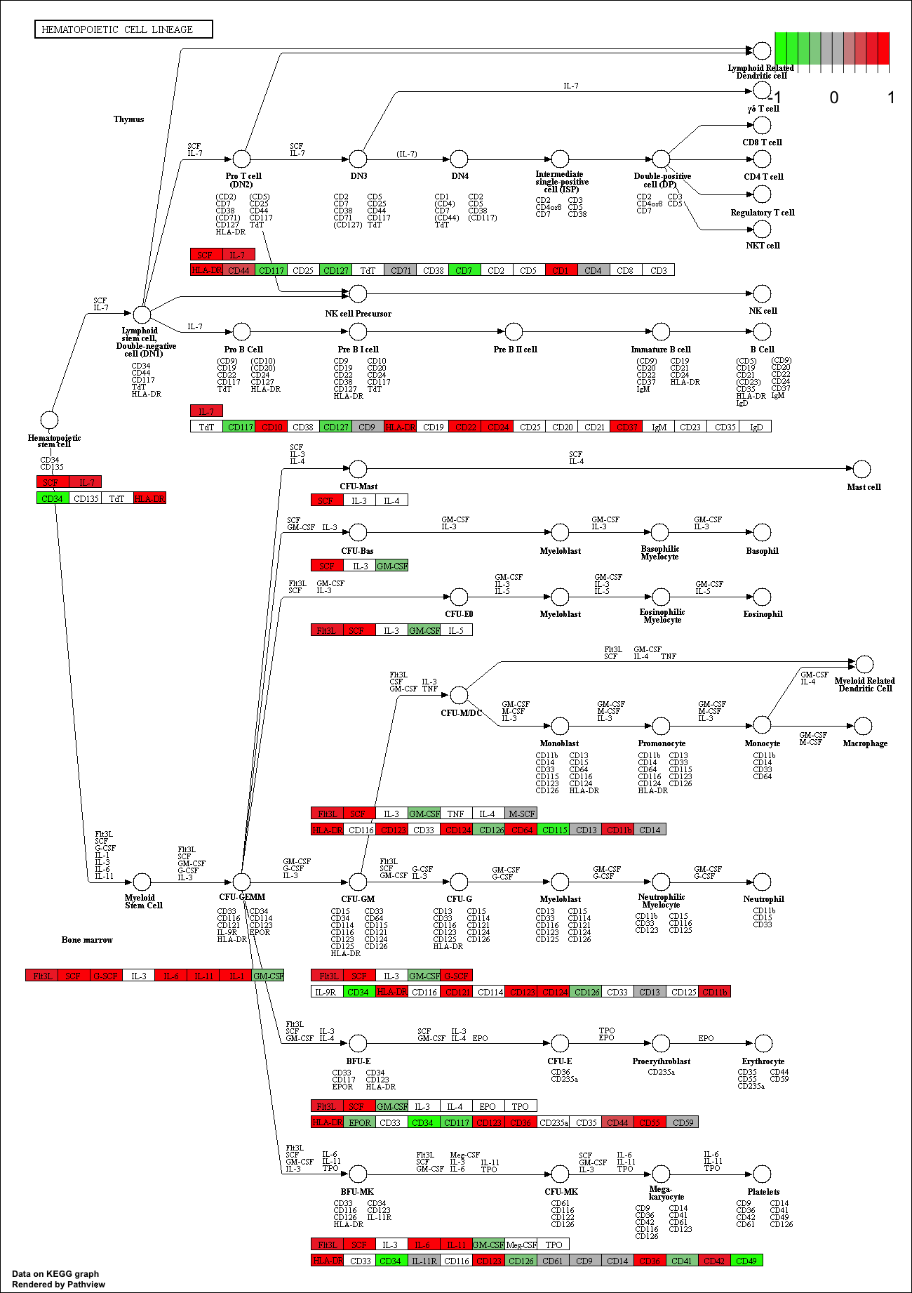
## hsa04640 Hematopoietic cell lineage 0.002709366 2.857393 0.002709366
## hsa04630 Jak-STAT signaling pathway 0.005655916 2.557207 0.005655916
## hsa04142 Lysosome 0.008948808 2.384783 0.008948808
## hsa00140 Steroid hormone biosynthesis 0.009619717 2.432105 0.009619717
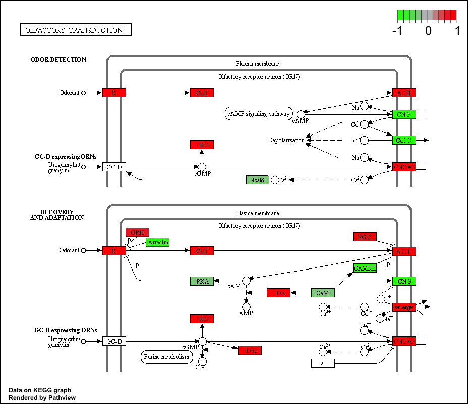
## hsa04740 Olfactory transduction 0.014450242 2.239717 0.014450242
## hsa04916 Melanogenesis 0.022339115 2.023074 0.022339115
## q.val set.size exp1
## hsa04640 Hematopoietic cell lineage 0.3847887 49 0.002709366
## hsa04630 Jak-STAT signaling pathway 0.3847887 103 0.005655916
## hsa04142 Lysosome 0.3847887 117 0.008948808
## hsa00140 Steroid hormone biosynthesis 0.3847887 26 0.009619717
## hsa04740 Olfactory transduction 0.4624078 39 0.014450242
## hsa04916 Melanogenesis 0.5297970 85 0.022339115
head(keggres$less)
##                                      p.geomean stat.mean        p.val
## hsa04110 Cell cycle               1.004024e-05 -4.353447 1.004024e-05
## hsa03030 DNA replication          8.909718e-05 -3.968605 8.909718e-05
## hsa03013 RNA transport            1.471026e-03 -3.007785 1.471026e-03
## hsa04114 Oocyte meiosis           1.987557e-03 -2.915377 1.987557e-03
## hsa03440 Homologous recombination 2.942017e-03 -2.868137 2.942017e-03
## hsa00240 Pyrimidine metabolism    5.800212e-03 -2.549616 5.800212e-03
##                                         q.val set.size         exp1
## hsa04110 Cell cycle               0.001606438      120 1.004024e-05
## hsa03030 DNA replication          0.007127774       36 8.909718e-05
## hsa03013 RNA transport            0.078454709      143 1.471026e-03
## hsa04114 Oocyte meiosis           0.079502292       98 1.987557e-03
## hsa03440 Homologous recombination 0.094144560       28 2.942017e-03
## hsa00240 Pyrimidine metabolism    0.138500584       95 5.800212e-03
Each keggres$greater and keggres$less object is data matrix with gene sets as rows sorted by p-value. Lets look at both up (greater), down (less), and statistics by calling head() with the lapply() function. As always if you want to find out more about a particular function or its return values use the R help system (e.g. ?gage or ?lapply).
lapply(keggres, head)
## $greater
##                                         p.geomean stat.mean       p.val
## hsa04640 Hematopoietic cell lineage   0.002709366  2.857393 0.002709366
## hsa04630 Jak-STAT signaling pathway   0.005655916  2.557207 0.005655916
## hsa04142 Lysosome                     0.008948808  2.384783 0.008948808
## hsa00140 Steroid hormone biosynthesis 0.009619717  2.432105 0.009619717
## hsa04740 Olfactory transduction       0.014450242  2.239717 0.014450242
## hsa04916 Melanogenesis                0.022339115  2.023074 0.022339115
##                                           q.val set.size        exp1
## hsa04640 Hematopoietic cell lineage   0.3847887       49 0.002709366
## hsa04630 Jak-STAT signaling pathway   0.3847887      103 0.005655916
## hsa04142 Lysosome                     0.3847887      117 0.008948808
## hsa00140 Steroid hormone biosynthesis 0.3847887       26 0.009619717
## hsa04740 Olfactory transduction       0.4624078       39 0.014450242
## hsa04916 Melanogenesis                0.5297970       85 0.022339115
##
## $less
##                                      p.geomean stat.mean        p.val
## hsa04110 Cell cycle               1.004024e-05 -4.353447 1.004024e-05
## hsa03030 DNA replication          8.909718e-05 -3.968605 8.909718e-05
## hsa03013 RNA transport            1.471026e-03 -3.007785 1.471026e-03
## hsa04114 Oocyte meiosis           1.987557e-03 -2.915377 1.987557e-03
## hsa03440 Homologous recombination 2.942017e-03 -2.868137 2.942017e-03
## hsa00240 Pyrimidine metabolism    5.800212e-03 -2.549616 5.800212e-03
##                                         q.val set.size         exp1
## hsa04110 Cell cycle               0.001606438      120 1.004024e-05
## hsa03030 DNA replication          0.007127774       36 8.909718e-05
## hsa03013 RNA transport            0.078454709      143 1.471026e-03
## hsa04114 Oocyte meiosis           0.079502292       98 1.987557e-03
## hsa03440 Homologous recombination 0.094144560       28 2.942017e-03
## hsa00240 Pyrimidine metabolism    0.138500584       95 5.800212e-03
##
## $stats
##                                       stat.mean     exp1
## hsa04640 Hematopoietic cell lineage    2.857393 2.857393
## hsa04630 Jak-STAT signaling pathway    2.557207 2.557207
## hsa04142 Lysosome                      2.384783 2.384783
## hsa00140 Steroid hormone biosynthesis  2.432105 2.432105
## hsa04740 Olfactory transduction        2.239717 2.239717
## hsa04916 Melanogenesis                 2.023074 2.023074
Now, let’s process the results to pull out the top 5 upregulated pathways, then further process that just to get the IDs. We’ll use these KEGG pathway IDs downstream for plotting.
## Sanity check displaying all pathways data
pathways = data.frame(id=rownames(keggres$greater), keggres$greater)
head(pathways)
##                                                                          id
## hsa04640 Hematopoietic cell lineage     hsa04640 Hematopoietic cell lineage
## hsa04630 Jak-STAT signaling pathway     hsa04630 Jak-STAT signaling pathway
## hsa04142 Lysosome                                         hsa04142 Lysosome
## hsa00140 Steroid hormone biosynthesis hsa00140 Steroid hormone biosynthesis
## hsa04740 Olfactory transduction             hsa04740 Olfactory transduction
## hsa04916 Melanogenesis                               hsa04916 Melanogenesis
##                                         p.geomean stat.mean       p.val
## hsa04640 Hematopoietic cell lineage   0.002709366  2.857393 0.002709366
## hsa04630 Jak-STAT signaling pathway   0.005655916  2.557207 0.005655916
## hsa04142 Lysosome                     0.008948808  2.384783 0.008948808
## hsa00140 Steroid hormone biosynthesis 0.009619717  2.432105 0.009619717
## hsa04740 Olfactory transduction       0.014450242  2.239717 0.014450242
## hsa04916 Melanogenesis                0.022339115  2.023074 0.022339115
##                                           q.val set.size        exp1
## hsa04640 Hematopoietic cell lineage   0.3847887       49 0.002709366
## hsa04630 Jak-STAT signaling pathway   0.3847887      103 0.005655916
## hsa04142 Lysosome                     0.3847887      117 0.008948808
## hsa00140 Steroid hormone biosynthesis 0.3847887       26 0.009619717
## hsa04740 Olfactory transduction       0.4624078       39 0.014450242
## hsa04916 Melanogenesis                0.5297970       85 0.022339115
Now, let’s try out the pathview() function from the pathview package to make a pathway plot with our result shown in color. To begin with lets manually supply a pathway.id (namely the first part of the "hsa04110 Cell cycle") that we could see from the print out above.
pathview(gene.data=foldchanges, pathway.id="hsa04110")
## Info: Downloading xml files for hsa04110, 1/1 pathways..
## Info: Downloading png files for hsa04110, 1/1 pathways..
## 'select()' returned 1:1 mapping between keys and columns
## Info: Working in directory /Users/barry/Desktop/bggn213_class/class18
## Info: Writing image file hsa04110.pathview.png
This downloads the patway figure data from KEGG and adds our results to it. You can play with the other input arguments to pathview() to change the dispay in various ways including generating a PDF graph. For example:
# A different PDF based output of the same data
pathview(gene.data=foldchanges, pathway.id="hsa04110", kegg.native=FALSE)
Here is the default low resolution raster PNG output from the first pathview() call above:
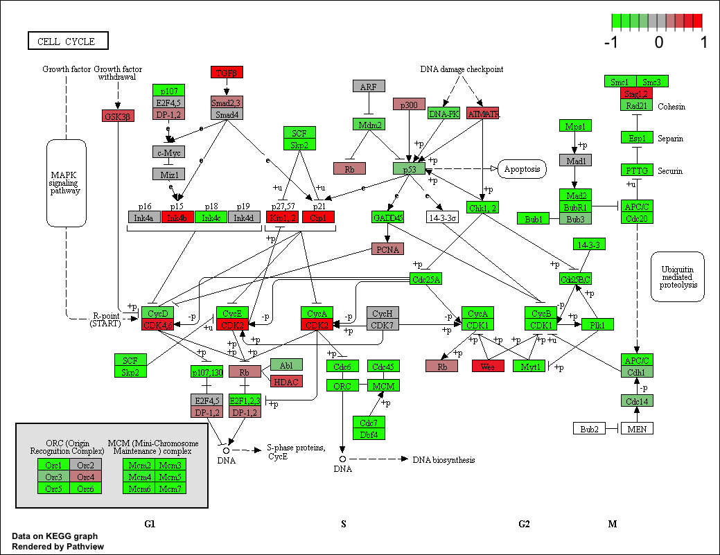
Note how many of the genes in this pathway are pertubed (i.e. colored) in our results.
Now, let’s process our results a bit more to automagicaly pull out the top 5 upregulated pathways, then further process that just to get the IDs needed by the pathview() function. We’ll use these KEGG pathway IDs for plotting below.
## Focus on top 5 upregulated pathways here for demo purposes only
keggrespathways <- rownames(keggres$greater)[1:5]

# Extract the IDs part of each string
keggresids = substr(keggrespathways, start=1, stop=8)
keggresids
## [1] "hsa04640" "hsa04630" "hsa04142" "hsa00140" "hsa04740"
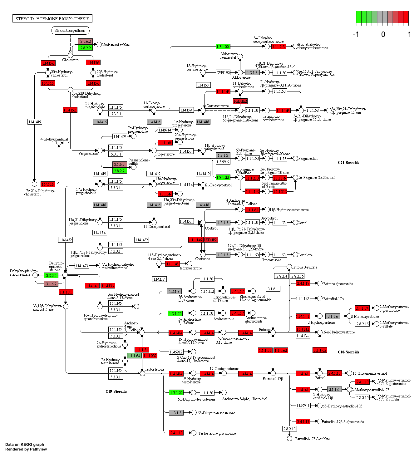
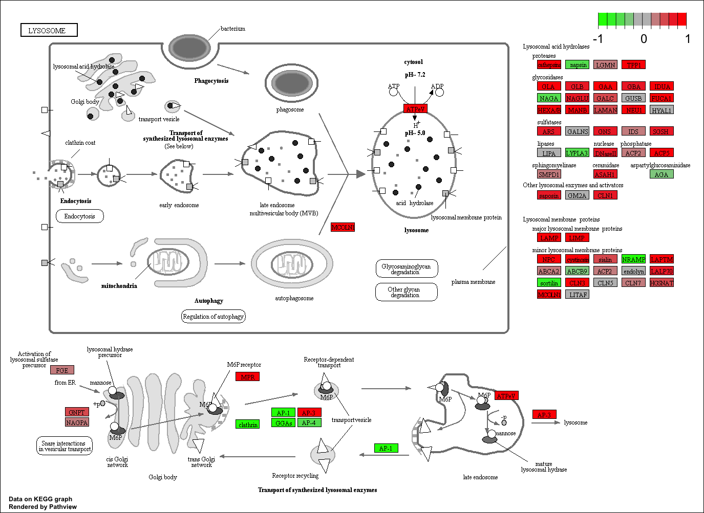
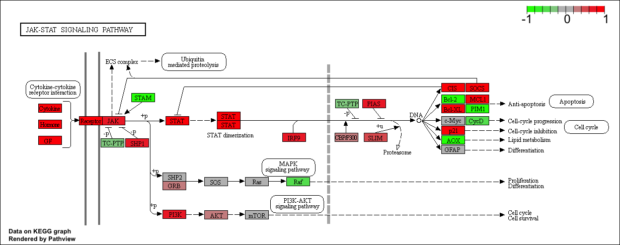
Finally, lets pass these IDs in keggresids to the pathview() function to draw plots for all the top 5 pathways.
pathview(gene.data=foldchanges, pathway.id=keggresids, species="hsa")
Here are the plots:
Section 3. Gene Ontology (GO)
We can also do a similar procedure with gene ontology. Similar to above, go.sets.hs has all GO terms. go.subs.hs is a named list containing indexes for the BP, CC, and MF ontologies. Let’s only do Biological Process.
data(go.sets.hs)
data(go.subs.hs)
gobpsets = go.sets.hs[go.subs.hs$BP]

gobpres = gage(foldchanges, gsets=gobpsets, same.dir=TRUE)

lapply(gobpres, head)
## $greater
##                                              p.geomean stat.mean
## GO:0007156 homophilic cell adhesion       4.893044e-05  3.971869
## GO:0060429 epithelium development         6.727999e-05  3.834578
## GO:0007610 behavior                       2.171759e-04  3.534089
## GO:0048729 tissue morphogenesis           2.471263e-04  3.498950
## GO:0002009 morphogenesis of an epithelium 3.227727e-04  3.429293
## GO:0016337 cell-cell adhesion             8.194676e-04  3.163087
##                                                  p.val     q.val set.size
## GO:0007156 homophilic cell adhesion       4.893044e-05 0.1337863      107
## GO:0060429 epithelium development         6.727999e-05 0.1337863      478
## GO:0007610 behavior                       2.171759e-04 0.2457053      404
## GO:0048729 tissue morphogenesis           2.471263e-04 0.2457053      403
## GO:0002009 morphogenesis of an epithelium 3.227727e-04 0.2567334      326
## GO:0016337 cell-cell adhesion             8.194676e-04 0.3753986      318
##                                                   exp1
## GO:0007156 homophilic cell adhesion       4.893044e-05
## GO:0060429 epithelium development         6.727999e-05
## GO:0007610 behavior                       2.171759e-04
## GO:0048729 tissue morphogenesis           2.471263e-04
## GO:0002009 morphogenesis of an epithelium 3.227727e-04
## GO:0016337 cell-cell adhesion             8.194676e-04
##
## $less
##                                             p.geomean stat.mean
## GO:0000279 M phase                       1.582159e-16 -8.314874
## GO:0048285 organelle fission             8.120979e-16 -8.149796
## GO:0000280 nuclear division              2.314155e-15 -8.024006
## GO:0007067 mitosis                       2.314155e-15 -8.024006
## GO:0000087 M phase of mitotic cell cycle 6.404776e-15 -7.881237
## GO:0007059 chromosome segregation        1.055849e-11 -6.988384
##                                                 p.val        q.val
## GO:0000279 M phase                       1.582159e-16 6.292245e-13
## GO:0048285 organelle fission             8.120979e-16 1.614857e-12
## GO:0000280 nuclear division              2.314155e-15 2.300848e-12
## GO:0007067 mitosis                       2.314155e-15 2.300848e-12
## GO:0000087 M phase of mitotic cell cycle 6.404776e-15 5.094359e-12
## GO:0007059 chromosome segregation        1.055849e-11 6.998521e-09
##                                          set.size         exp1
## GO:0000279 M phase                            492 1.582159e-16
## GO:0048285 organelle fission                  373 8.120979e-16
## GO:0000280 nuclear division                   349 2.314155e-15
## GO:0007067 mitosis                            349 2.314155e-15
## GO:0000087 M phase of mitotic cell cycle      359 6.404776e-15
## GO:0007059 chromosome segregation             141 1.055849e-11
##
## $stats
##                                           stat.mean     exp1
## GO:0007156 homophilic cell adhesion        3.971869 3.971869
## GO:0060429 epithelium development          3.834578 3.834578
## GO:0007610 behavior                        3.534089 3.534089
## GO:0048729 tissue morphogenesis            3.498950 3.498950
## GO:0002009 morphogenesis of an epithelium  3.429293 3.429293
## GO:0016337 cell-cell adhesion              3.163087 3.163087
Section 4. Reactome Pathway Analysis
Reactome is database consisting of biological molecules and their relation to pathways and processes. Reactome, such as many other tools, has an online software available (https://reactome.org/) and R package available (https://bioconductor.org/packages/release/bioc/html/ReactomePA.html).
If you would like more information, the documentation is available here: https://reactome.org/user/guide
Let’s now conduct over-representation enrichment analysis and pathway-topology analysis with Reactome using the previous list of significant genes generated from our differential expression results above.
First, Using R, output the list of significant genes at the 0.05 level as a plain text file:
sig_genes <- res[res$padj <= 0.05 & !is.na(res$padj), "symbol"]
print(paste("Total number of significant genes:", length(sig_genes)))
## [1] "Total number of significant genes: 8151"
write.table(sig_genes, file="significant_genes.txt", row.names=FALSE, col.names=FALSE, quote=FALSE)
Then, to perform pathway analysis online go to the Reactome website (https://reactome.org/PathwayBrowser/#TOOL=AT). Select “choose file” to upload your significant gene list. Then, select the parameters “Project to Humans”, then click “Analyze”.
Question: What pathway has the most significant “Entities p-value”? Do the most significant pathways listed match your previous KEGG results? What factors could cause differences between the two methods?
Section 5. GO Analysis
Gene Set Gene Ontology (GO) Enrichment is a method to determine over-represented or under-represented GO terms for a given set of genes. GO terms are formal structured controlled vocabularies (ontologies) for gene products in terms of their biological function. The goal of this analysis is to determine the biological process the given set of genes are associated with.
To perform Gene Set GO Enrichment online go to the website http://www.geneontology.org/page/go-enrichment-analysis. Paste your significant gene list from section 4. Then, select “biological process” and “homo sapiens”, and click submit.
Question: What pathway has the most significant “Entities p-value”? Do the most significant pathways listed match your previous KEGG results? What factors could cause differences between the two methods?
Session Information
The sessionInfo() prints version information about R and any attached packages. It’s a good practice to always run this command at the end of your R session and record it for the sake of reproducibility in the future.
sessionInfo()
## R version 3.4.1 (2017-06-30)
## Platform: x86_64-apple-darwin15.6.0 (64-bit)
## Running under: macOS Sierra 10.12.6
##
## Matrix products: default
## BLAS: /Library/Frameworks/R.framework/Versions/3.4/Resources/lib/libRblas.0.dylib
## LAPACK: /Library/Frameworks/R.framework/Versions/3.4/Resources/lib/libRlapack.dylib
##
## locale:
## [1] en_US.UTF-8/en_US.UTF-8/en_US.UTF-8/C/en_US.UTF-8/en_US.UTF-8
##
## attached base packages:
## [1] parallel  stats4    stats     graphics  grDevices utils     datasets
## [8] methods   base
##
## other attached packages:
##  [1] gageData_2.16.0            gage_2.28.0
##  [3] pathview_1.18.0            org.Hs.eg.db_3.5.0
##  [5] AnnotationDbi_1.40.0       DESeq2_1.18.1
##  [7] SummarizedExperiment_1.8.0 DelayedArray_0.4.1
##  [9] matrixStats_0.52.2         Biobase_2.38.0
## [11] GenomicRanges_1.30.0       GenomeInfoDb_1.14.0
## [13] IRanges_2.12.0             S4Vectors_0.16.0
## [15] BiocGenerics_0.24.0
##
## loaded via a namespace (and not attached):
##  [1] httr_1.3.1              bit64_0.9-7
##  [3] splines_3.4.1           Formula_1.2-2
##  [5] latticeExtra_0.6-28     blob_1.1.0
##  [7] GenomeInfoDbData_0.99.1 yaml_2.1.14
##  [9] RSQLite_2.0             backports_1.1.1
## [11] lattice_0.20-35         digest_0.6.12
## [13] RColorBrewer_1.1-2      XVector_0.18.0
## [15] checkmate_1.8.5         colorspace_1.3-2
## [17] htmltools_0.3.6         Matrix_1.2-12
## [19] plyr_1.8.4              XML_3.98-1.9
## [21] pkgconfig_2.0.1         genefilter_1.60.0
## [23] zlibbioc_1.24.0         xtable_1.8-2
## [25] scales_0.5.0            BiocParallel_1.12.0
## [27] htmlTable_1.9           tibble_1.3.4
## [29] annotate_1.56.1         KEGGREST_1.18.0
## [31] ggplot2_2.2.1           nnet_7.3-12
## [33] lazyeval_0.2.1          survival_2.41-3
## [35] magrittr_1.5            memoise_1.1.0
## [37] evaluate_0.10.1         KEGGgraph_1.38.0
## [39] foreign_0.8-69          graph_1.56.0
## [41] tools_3.4.1             data.table_1.10.4-3
## [43] stringr_1.2.0           munsell_0.4.3
## [45] locfit_1.5-9.1          cluster_2.0.6
## [47] Biostrings_2.46.0       compiler_3.4.1
## [49] rlang_0.1.4             grid_3.4.1
## [51] RCurl_1.95-4.8          htmlwidgets_0.9
## [53] bitops_1.0-6            base64enc_0.1-3
## [55] rmarkdown_1.8           gtable_0.2.0
## [57] DBI_0.7                 R6_2.2.2
## [59] gridExtra_2.3           knitr_1.17
## [61] bit_1.1-12              Hmisc_4.0-3
## [63] rprojroot_1.2           Rgraphviz_2.22.0
## [65] stringi_1.1.6           Rcpp_0.12.13
## [67] png_0.1-7               geneplotter_1.56.0
## [69] rpart_4.1-11            acepack_1.4.1