Visualization with R Lecture (Part 1)
Circle points function
Lets write a wee function to create some points on the circumference of a circle. We will use the equation of a circle with origin (j, k) and radius r: x(t) = r cos(t) + j and y(t) = r sin(t) + k See for example: http://www.math.com/tables/geometry/circles.htm
cpoints <- function(radius=5, center=c(0,0), angle=seq(0,360,length=15)) {
  return( cbind( x=radius*cos(angle)+center[1],
                 y=radius*sin(angle)+center[2] ))
}
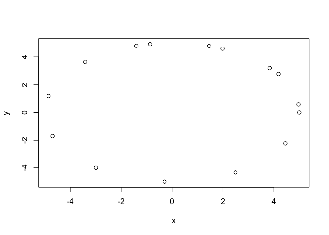
Lets print out p and make a quick plot
p <- cpoints()
p
##                x          y
##  [1,]  5.0000000  0.0000000
##  [2,]  4.1780762  2.7465759
##  [3,]  1.9825283  4.5901614
##  [4,] -0.8648146  4.9246417
##  [5,] -3.4278327  3.6400499
##  [6,] -4.8638839  1.1587206
##  [7,] -4.7008383 -1.7035607
##  [8,] -2.9923003 -4.0057632
##  [9,] -0.2999852 -4.9909928
## [10,]  2.4909559 -4.3353360
## [11,]  4.4629466 -2.2543529
## [12,]  4.9676565  0.5677927
## [13,]  3.8391523  3.2032654
## [14,]  1.4484519  4.7856021
## [15,] -1.4184555  4.7945786
plot( p )
Calculate some summary statistics for x and y. Note here we use the apply() function to call the summary() function on the cols by setting the margin=2 argument. What would setting `margin=1 return?
apply(p, 2, summary)
##                  x          y
## Min.    -4.8638839 -4.9909928
## 1st Qu. -2.2053779 -1.9789568
## Median   1.4484519  1.1587206
## Mean     0.6534438  0.8747588
## 3rd Qu.  4.0086143  4.1151056
## Max.     5.0000000  4.9246417
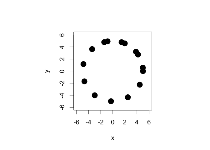
Tidy the figure
Lets make the plot square and increase axis font sizes, change ploting character and increase its size.
par(pty="s", cex=1.3)
plot(p, xlim=c(-6,6), ylim=c(-6,6), xlab="x", ylab="y", pch=16, cex=2)
For my lecture slides I will make a PDF and have the points and font in white with transparent background (the default when we save a PDF from code rather than the RStudio Export button).
pdf(file="Rplot.pdf")
par(pty="s", cex=1.3)
plot(p, xlim=c(-6,6), ylim=c(-6,6), xlab="x", ylab="y", col="white", col.axis="white", col.lab="white", pch=16, cex=2)
dev.off()
## quartz_off_screen
##                 2
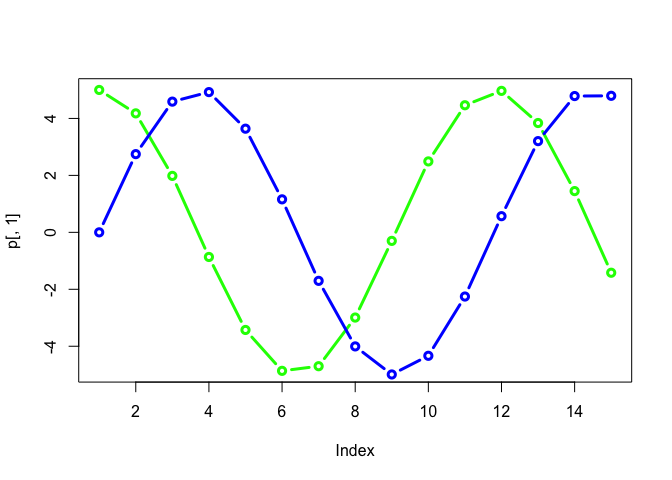
Non optimal plot in this instance
But showing it as a time-series obscures the relationship. This is still better than a simple table.
plot(p[,1], typ="b", col="green", lwd=3)
points(p[,2], typ="b", col="blue", lwd=3)
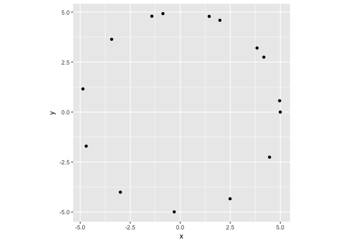
Or we can use ggplot2 but note that ggplot2 needs a data.frame object as input!
library(ggplot2)
pc <- as.data.frame(p)
ggplot(pc, aes(x,y)) + geom_point() + coord_equal()
For some other plots in this lecture (i.e. Part 2.) we will use the more complicated but more versitile ggplot2 package. We will cover the basics of ggplot later.
Side-Note: GitHub Documents
This is an R Markdown format used for publishing markdown documents to GitHub. You can create your own from within RStudio via File > New File > RMarkdown > From Template. Then when you click the Knit button in RStudio all R code chunks are run and a markdown file (.md) suitable for publishing to GitHub is generated.
Session Information
sessionInfo()
## R version 3.4.1 (2017-06-30)
## Platform: x86_64-apple-darwin15.6.0 (64-bit)
## Running under: macOS Sierra 10.12.6
##
## Matrix products: default
## BLAS: /Library/Frameworks/R.framework/Versions/3.4/Resources/lib/libRblas.0.dylib
## LAPACK: /Library/Frameworks/R.framework/Versions/3.4/Resources/lib/libRlapack.dylib
##
## locale:
## [1] en_US.UTF-8/en_US.UTF-8/en_US.UTF-8/C/en_US.UTF-8/en_US.UTF-8
##
## attached base packages:
## [1] stats     graphics  grDevices utils     datasets  methods   base
##
## other attached packages:
## [1] ggplot2_2.2.1
##
## loaded via a namespace (and not attached):
##  [1] Rcpp_0.12.13     digest_0.6.12    rprojroot_1.2    plyr_1.8.4
##  [5] grid_3.4.1       gtable_0.2.0     backports_1.1.1  magrittr_1.5
##  [9] evaluate_0.10.1  scales_0.5.0     rlang_0.1.2      stringi_1.1.5
## [13] lazyeval_0.2.0   rmarkdown_1.6    labeling_0.3     tools_3.4.1
## [17] stringr_1.2.0    munsell_0.4.3    yaml_2.1.14      compiler_3.4.1
## [21] colorspace_1.3-2 htmltools_0.3.6  knitr_1.17       tibble_1.3.4