BIMM-143, Lecture 09
Hands-on with unsupervised learning analysis of cancer cells
Background
The goal of this hands-on session is for you to explore a complete analysis using the unsupervised learning techniques covered in the last class. You’ll extend what you’ve learned by combining PCA as a preprocessing step to clustering using data that consist of measurements of cell nuclei of human breast masses. This expands on our RNA-Seq analysis from last day.
The data itself comes from the Wisconsin Breast Cancer Diagnostic Data Set first reported by K. P. Benne and O. L. Mangasarian: “Robust Linear Programming Discrimination of Two Linearly Inseparable Sets”.
Values in this data set describe characteristics of the cell nuclei present in digitized images of a fine needle aspiration (FNA) of a breast mass. For example radius (i.e. mean of distances from center to points on the perimeter), texture (i.e. standard deviation of gray-scale values), and smoothness (local variation in radius lengths). Summary information is also provided for each group of cells including diagnosis (i.e. benign (not cancerous) and and malignant (cancerous)).
Section 1.
Preparing the data
Before we can begin our analysis we first have to download and import our data correctly into our R session.
For this we can use the read.csv() function to read the CSV (comma-separated values) file containing the data from the URL: https://bioboot.github.io/bimm143_W18/class-material/WisconsinCancer.csv
Assign the result to an object called wisc.df.
url <- "https://bioboot.github.io/bimm143_W18/class-material/WisconsinCancer.csv"

# Complete the following code to input the data and store as wisc.df
wisc.df <- ___
Examine your input data to ensure column names are set correctly. The id and diagnosis columns will not be used for most of the following steps. Use as.matrix() to convert the other features (i.e. columns) of the data (in columns 3 through 32) to a matrix. Store this in a variable called wisc.data.
# Convert the features of the data: wisc.data
wisc.data <- as.matrix( ___ )
Assign the row names of wisc.data the values currently contained in the id column of wisc.df. While not strictly required, this will help you keep track of the different observations throughout the modeling process.
# Set the row names of wisc.data
row.names(wisc.data) <- wisc.df$id
#head(wisc.data)
Finally, setup a separate new vector called diagnosis to be 1 if a diagnosis is malignant ("M") and 0 otherwise. Note that R coerces TRUE to 1 and FALSE to 0.
# Create diagnosis vector by completing the missing code
diagnosis <- as.numeric( ___ )
Exploratory data analysis
The first step of any data analysis, unsupervised or supervised, is to familiarize yourself with the data.
Explore the data you created before (wisc.data and diagnosis) to answer the following questions:
- Q1. How many observations are in this dataset?
- Q2. How many variables/features in the data are suffixed with
_mean? - Q3. How many of the observations have a malignant diagnosis?
The functions
dim(),length(),grep()andsum()may be useful for answering the first 3 questions above.
Section 2.
Performing PCA
The next step in your analysis is to perform principal component analysis (PCA) on wisc.data.
It is important to check if the data need to be scaled before performing PCA. Recall two common reasons for scaling data include:
- The input variables use different units of measurement.
- The input variables have significantly different variances.
Check the mean and standard deviation of the features (i.e. columns) of the wisc.data to determine if the data should be scaled. Use the colMeans() and apply() functions like you’ve done before.
# Check column means and standard deviations
colMeans(wisc.data)

apply(wisc.data,2,sd)
Execute PCA with the prcomp() function on the wisc.data, scaling if appropriate, and assign the output model to wisc.pr.
# Perform PCA on wisc.data by completing the following code
wisc.pr <- prcomp( ___ )
Inspect a summary of the results with the summary() function.
# Look at summary of results
summary(wisc.pr)
## Importance of components%s:
##                           PC1    PC2     PC3     PC4     PC5     PC6
## Standard deviation     3.6444 2.3857 1.67867 1.40735 1.28403 1.09880
## Proportion of Variance 0.4427 0.1897 0.09393 0.06602 0.05496 0.04025
## Cumulative Proportion  0.4427 0.6324 0.72636 0.79239 0.84734 0.88759
##                            PC7     PC8    PC9    PC10   PC11    PC12
## Standard deviation     0.82172 0.69037 0.6457 0.59219 0.5421 0.51104
## Proportion of Variance 0.02251 0.01589 0.0139 0.01169 0.0098 0.00871
## Cumulative Proportion  0.91010 0.92598 0.9399 0.95157 0.9614 0.97007
##                           PC13    PC14    PC15    PC16    PC17    PC18
## Standard deviation     0.49128 0.39624 0.30681 0.28260 0.24372 0.22939
## Proportion of Variance 0.00805 0.00523 0.00314 0.00266 0.00198 0.00175
## Cumulative Proportion  0.97812 0.98335 0.98649 0.98915 0.99113 0.99288
##                           PC19    PC20   PC21    PC22    PC23   PC24
## Standard deviation     0.22244 0.17652 0.1731 0.16565 0.15602 0.1344
## Proportion of Variance 0.00165 0.00104 0.0010 0.00091 0.00081 0.0006
## Cumulative Proportion  0.99453 0.99557 0.9966 0.99749 0.99830 0.9989
##                           PC25    PC26    PC27    PC28    PC29    PC30
## Standard deviation     0.12442 0.09043 0.08307 0.03987 0.02736 0.01153
## Proportion of Variance 0.00052 0.00027 0.00023 0.00005 0.00002 0.00000
## Cumulative Proportion  0.99942 0.99969 0.99992 0.99997 1.00000 1.00000
- Q4. From your results, what proportion of the original variance is captured by the first principal components (PC1)?
- Q5. How many principal components (PCs) are required to describe at least 70% of the original variance in the data?
- Q6. How many principal components (PCs) are required to describe at least 90% of the original variance in the data?
Interpreting PCA results
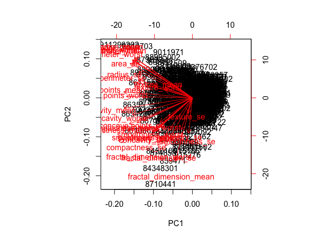
Now you will use some visualizations to better understand your PCA model. You were introduced to one of these visualizations, the biplot, last day.
You will often run into some common challenges with using biplots on real-world data containing a non-trivial number of observations and variables, then you’ll look at some alternative visualizations. You are encouraged to experiment with additional visualizations before moving on to the next section
Create a biplot of the wisc.pr using the biplot() function.
- Q7. What stands out to you about this plot? Is it easy or difficult to understand? Why?
biplot(wisc.pr)
# Scatter plot observations by components 1 and 2
plot( ___ , col = ___ ,
     xlab = "PC1", ylab = "PC2")
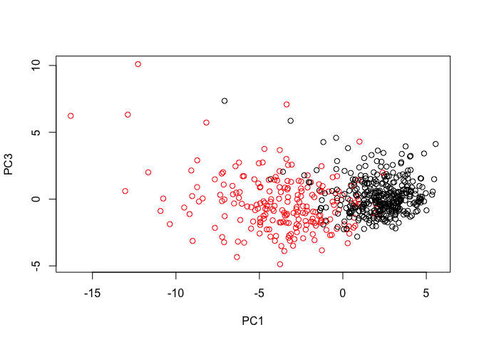
- Q8. Repeat the same for principal components 1 and 3. What do you notice about these plots?
# Repeat for components 1 and 3
plot(wisc.pr$x[, c(1, 3)], col = (diagnosis + 1),
     xlab = "PC1", ylab = "PC3")
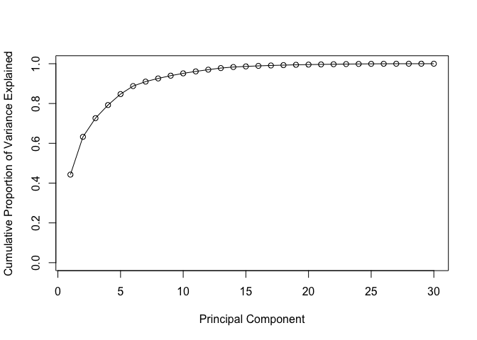
Using the cumsum() function, create a plot of cumulative proportion of variance explained.
# Plot cumulative proportion of variance explained
plot(cumsum(pve), xlab = "Principal Component",
     ylab = "Cumulative Proportion of Variance Explained",
     ylim = c(0, 1), type = "o")
Communicating PCA results
In this section we will check your understanding of the PCA results, in particular the loadings and variance explained. The loadings, represented as vectors, explain the mapping from the original features to the principal components. The principal components are naturally ordered from the most variance explained to the least variance explained.
Q9. For the first principal component, what is the component of the loading vector (i.e.
wisc.pr$rotation[,1]) for the featureconcave.points_mean?Q10. What is the minimum number of principal components required to explain 80% of the variance of the data?
Section 3.
Hierarchical clustering of case data
The goal of this section is to do hierarchical clustering of the observations. Recall from our last class that this type of clustering does not assume in advance the number of natural groups that exist in the data.
As part of the preparation for hierarchical clustering, the distance between all pairs of observations are computed. Furthermore, there are different ways to link clusters together, with single, complete, and average being the most common linkage methods.
Scale the wisc.data data and assign the result to data.scaled.
# Scale the wisc.data data: data.scaled
data.scaled <- ___(wisc.data)
Calculate the (Euclidean) distances between all pairs of observations in the new scaled dataset and assign the result to data.dist.
data.dist <- ___(data.scaled)
Create a hierarchical clustering model using complete linkage. Manually specify the method argument to hclust() and assign the results to wisc.hclust.
wisc.hclust <- ___(data.dist, ___)
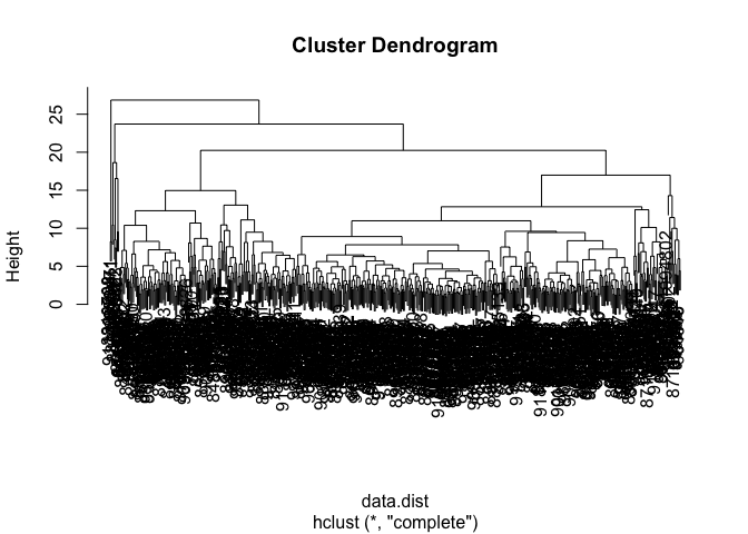
Results of hierarchical clustering
Let’s use the hierarchical clustering model you just created to determine a height (or distance between clusters) where a certain number of clusters exists.
- Q11. Using the
plot()function, what is the height at which the clustering model has 4 clusters?
plot(wisc.hclust)